2  Curvature and Torsion

We have seen how to describe curves and reparametrized them. Now we want to look at local properties of curves:

• How much does a curve twist?
• How much does a curve bend?

We will measure two quantities:

• Curvature: measures how much a curve $\gamma \gamma$ deviates from a straight line.
• Torsion: measures how much a curve $\gamma \gamma$ fails to lie on a plane.

For example a 2D spiral is curved, but still lies in a plane. Instead the Helix both deviates from a straight line and pulls away from any fixed plane.

2.1 Curvature

We start with an informal discussion. Suppose $\gamma \gamma$ is a straight line $$\gamma \gamma (t)=\mathbf{a}+t\mathbf{v}$$ with $\mathbf{a},\mathbf{v}\in {\mathbb{R}}^3$. The tangent vector to $\gamma \gamma$ is constant $$\dot{\gamma \gamma }(t)=\mathbf{v}.$$ Whatever the definition of curvature will be, it has to hold that $\gamma \gamma$ has zero curvature in this case. If we further derive the tangent vector, we obtain $$\ddot{\gamma \gamma }(t)=00.$$ Thus $\ddot{\gamma \gamma }$ seems to be a good candidate for the definition of curvature of $\gamma \gamma$ at the point $\gamma \gamma (t)$.

Suppose now that $\gamma \gamma$ is a curve in ${\mathbb{R}}^2$ with unit speed. We have proven that in this case $$\dot{\gamma \gamma }\cdot \ddot{\gamma \gamma }=0,$$ that is, the vector $\ddot{\gamma \gamma }$ is orthogonal to the tangent $\dot{\gamma \gamma }$ at all times. Now let $\mathbf{n}(t)$ be the unit vector orthogonal to $\dot{\gamma \gamma }(t)$ at the point $\gamma \gamma (t)$. The amount that the curve $\gamma \gamma$ deviates from its tangent at $\gamma \gamma (t)$ after time $t_0$ is $$\begin{array}{}\text{(2.1)}& (\gamma \gamma (t+t_0)-\gamma \gamma (t))\cdot \mathbf{n}(t),\end{array}$$ as seen in the figure below.

Amount that $\gamma \gamma$ deviates from tangent is $(\gamma \gamma (t+t_0)-\gamma \gamma (t))\cdot \mathbf{n}(t)$

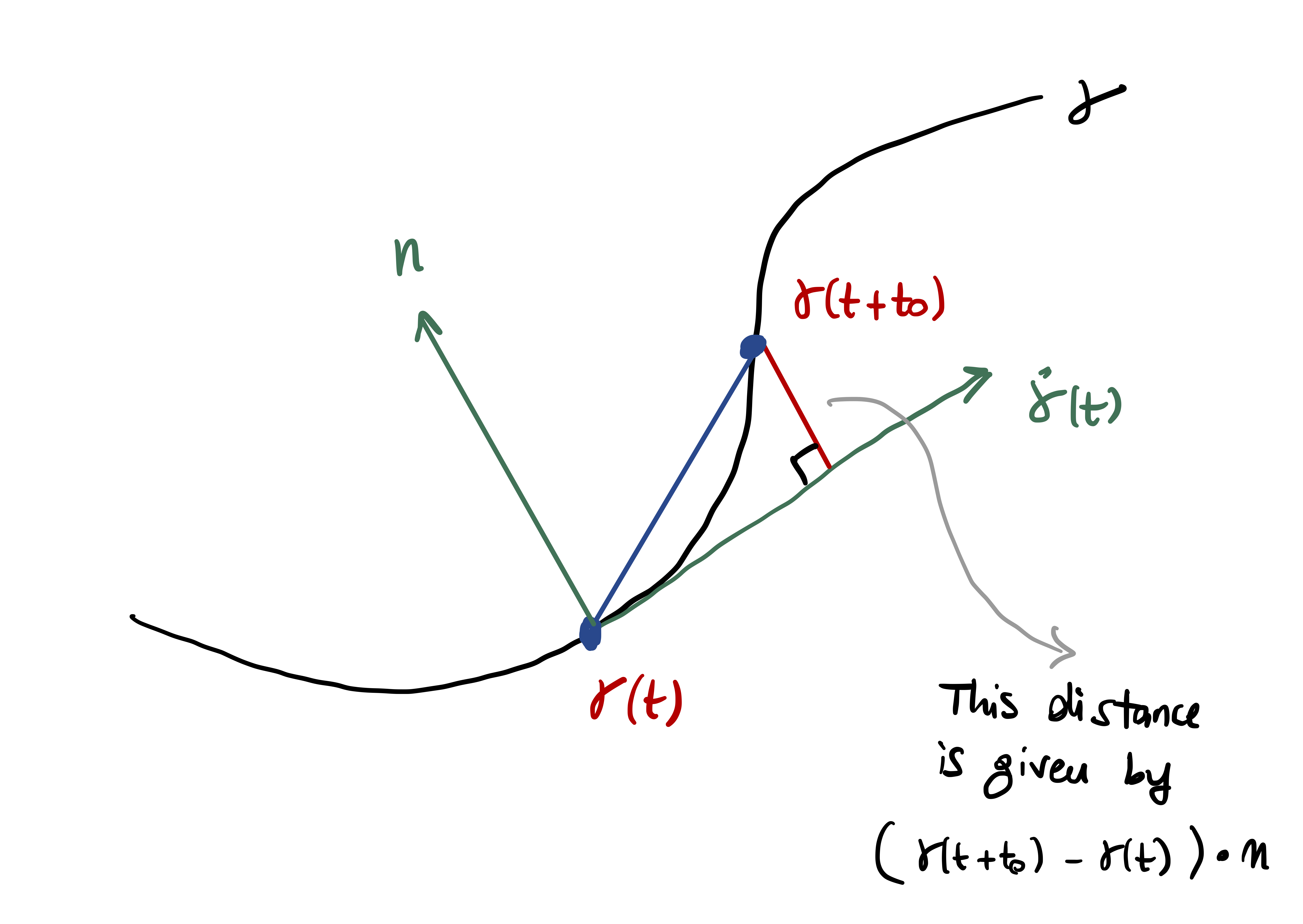
Equation (2.1) is what we take as measure of curvature. Since $$\dot{\gamma \gamma }(t)\cdot \ddot{\gamma \gamma }(t)=0\text{ and }\dot{\gamma \gamma }(t)\cdot \mathbf{n}(t)=0,$$ we conclude that $\ddot{\gamma \gamma }(t)$ is parallel to $\mathbf{n}(t)$. Since $\mathbf{n}(t)$ is a unit vector, there exists a scalar $\kappa (t)$ such that $$\ddot{\gamma \gamma }(t)=\kappa (t)\mathbf{n}(t).$$ As $\mathbf{n}$ is unitary, we have $$\kappa (t)=\Vert \ddot{\gamma \gamma }(t)\Vert$$

Now, approximate $\gamma \gamma$ at $t$ with its second order Taylor polynomial: $$\gamma \gamma (t+t_0)=\gamma \gamma (t)+\dot{\gamma \gamma }(t)t_0+\frac{\ddot{\gamma \gamma }(t)}{2}{t}_0^2+o(t_0)$$ where the remainder $o(t_0)$ is such that $$\underset{t_0\to 0}{lim}\frac{o(t_0)}{t_0^2}=0.$$ Therefore, discarding the remainder, $$\gamma \gamma (t+t_0)-\gamma \gamma (t)\approx \dot{\gamma \gamma }(t)t_0+\frac{\ddot{\gamma \gamma }(t)}{2}{t}_0^2.$$ Multiplying by $\mathbf{n}(t)$ we get $$(\gamma \gamma (t+t_0)-\gamma \gamma (t))\cdot \mathbf{n}(t)\approx \dot{\gamma \gamma }(t)\cdot \mathbf{n}(t)t_0+\frac{\ddot{\gamma \gamma }(t)\cdot \mathbf{n}(t)}{2}{t}_0^2.$$ Recalling that $$\dot{\gamma \gamma }(t)\cdot \mathbf{n}(t)=0,\ddot{\gamma \gamma }(t)\cdot \mathbf{n}(t)=\kappa (t),$$ we then obtain $$(\gamma \gamma (t+t_0)-\gamma \gamma (t))\cdot \mathbf{n}(t)\approx \frac{1}{2}\kappa (t)t_0^2$$

Important

The amount that $\gamma \gamma$ deviates from a straight line is proportional to $$\kappa (t)=\Vert \ddot{\gamma \gamma }(t)\Vert .$$

We take this as definition of curvature for a general unit speed curve in ${\mathbb{R}}^n.$

Definition 1

Let $\gamma \gamma :(a,b)\to {\mathbb{R}}^n$ be a unit speed curve. The curvature of $\gamma \gamma$ at $\gamma \gamma (t)$ is $${\kappa }^{\gamma \gamma }(t):=\Vert \ddot{\gamma \gamma }(t)\Vert .$$

Note that $\kappa (t)$ is a function of time. Therefore the curvature of $\gamma \gamma$ can change from point to point.

We now define curvature for curves which are regular, but not necessarily unit speed.

Definition 2

Let $\gamma \gamma :(a,b)\to {\mathbb{R}}^n$ be a regular. The curvature of $\gamma \gamma$ at $\gamma \gamma (t)$ is $${\kappa }^{\gamma \gamma }(t):=\Vert \ddot{\widetilde{\gamma \gamma }}(\varphi (t))\Vert ,\mathrm{\forall }t\in (a,b),$$ where $\widetilde{\gamma \gamma }$ is a unit speed reparametrization of $\gamma \gamma$, with $\gamma \gamma =\widetilde{\gamma \gamma }\circ \varphi$.

Remark 3

The above definition is well posed:

• Since $\gamma \gamma$ is regular, there exist a unit speed reparametrization $\widetilde{\gamma \gamma }$ of $\gamma \gamma$.
• If $\widehat{\gamma \gamma }$ is another unit speed reaprametrization of $\gamma \gamma$, with $\gamma \gamma =\widehat{\gamma \gamma }\circ \hat{\varphi }$, then $${\kappa }^{\gamma \gamma }(t)=\Vert \ddot{\widehat{\gamma \gamma }}(\hat{\varphi }(t))\Vert ,$$ showing that there is no ambiguity in the definition of ${\kappa }^{\gamma \gamma }$.

Indeed, since $\widetilde{\gamma \gamma }$ and $\widehat{\gamma \gamma }$ are both reparametrizations of $\gamma \gamma$, then $$\gamma \gamma (t)=\widetilde{\gamma \gamma }(\tilde{\varphi }(t)),\gamma \gamma (t)=\widehat{\gamma \gamma }(\hat{\varphi }(t))$$ for some diffeomorphisms $\tilde{\varphi },\hat{\varphi }$. Hence $$\begin{array}{}\text{(2.2)}& \widetilde{\gamma \gamma }(t)=\widehat{\gamma \gamma }(\varphi (t)),\varphi :=\hat{\varphi }\circ (\tilde{\varphi }{)}^{-1},\end{array}$$ where $\varphi$ is a diffeomorphism, since it is composition of diffeomorphisms. Differentiating (2.2) we get $$\begin{array}{}\text{(2.3)}& \dot{\widetilde{\gamma \gamma }}(t)=\dot{\widehat{\gamma \gamma }}(\varphi (t))\dot{\varphi }(t).\end{array}$$ Taking the norms of the above, and recalling that $\widetilde{\gamma \gamma }$ and $\widehat{\gamma \gamma }$ are unit speed, we get $$\begin{array}{}\text{(2.4)}& |\dot{\varphi }(t)|=1,\mathrm{\forall }t.\end{array}$$ Since $\varphi$ is a diffeomorphism, we already know that $|\dot{\varphi }|\ne 0$. As $\dot{\varphi }$ is continuous, this means that the sign of $\dot{\varphi }$ is constant. Thus (2.4) implies $$\dot{\varphi }(t)\equiv 1\text{or}\dot{\varphi }(t)\equiv -1.$$ In both cases, we have $$\ddot{\varphi }\equiv 0.$$ Differentiating (2.3) we then obtain $$\begin{array}{rl}\ddot{\widetilde{\gamma \gamma }}(t)& =\ddot{\widehat{\gamma \gamma }}(\varphi (t)){\dot{\varphi }}^2(t)+\dot{\widehat{\gamma \gamma }}(\varphi (t))\ddot{\varphi }(t)\\ & =\ddot{\widehat{\gamma \gamma }}(\varphi (t)){\dot{\varphi }}^2(t).\end{array}$$ Taking the norms and using again that $|\dot{\varphi }|\equiv 1$, we get that $$\Vert \ddot{\widetilde{\gamma \gamma }}(t)\Vert =\Vert \ddot{\widehat{\gamma \gamma }}(\varphi (t))\Vert .$$ Recalling that $\varphi =\hat{\varphi }\circ (\tilde{\varphi }{)}^{-1}$ we get $$\Vert \ddot{\widetilde{\gamma \gamma }}(\tilde{\varphi }(t))\Vert =\Vert \ddot{\widehat{\gamma \gamma }}(\hat{\varphi }(t))\Vert ,\mathrm{\forall }t\in (a,b).$$ Therefore $${\kappa }^{\gamma \gamma }(t)=\Vert \ddot{\widetilde{\gamma \gamma }}(\tilde{\varphi }(t))\Vert =\Vert \ddot{\widehat{\gamma \gamma }}(\hat{\varphi }(t))\Vert .$$

Remark 4: Methods for computing curvature

In summary, the curvature of a regular curve $$\gamma \gamma :(a,b)\to {\mathbb{R}}^n$$ is defined via unit speed reparametrizations of $\gamma \gamma$. To compute $\kappa$ we do the following:

• We find a unit speed reparametrization $\widetilde{\gamma \gamma }$ of the regular curve $\gamma \gamma$
• This can be done by computing $s$ the arc-length of $\gamma \gamma$, and then defining $$\widetilde{\gamma \gamma }:=\gamma \gamma \circ \psi ,\psi :=s^{-1}$$
• Then we compute $${\kappa }^{\widetilde{\gamma \gamma }}(t)=\Vert \ddot{\widetilde{\gamma \gamma }}\Vert (t)$$
• We obtain the curvature of $\gamma \gamma$ by $${\kappa }^{\gamma \gamma }(t)={\kappa }^{\widetilde{\gamma \gamma }}(t)$$

When $\gamma \gamma$ is regular and has values in ${\mathbb{R}}^3$, there is a way to compute $\kappa$ without reparametrizing. To do this, we will need the notion of cross product, or vector product. We will see this in the following sections.

Procedure for computing curvature $\kappa$

We conclude with two examples in which we compute the curvature $\kappa$ using unit speed reparametrizations.

Example 5

Consider the circle of radius $R>0$: $$\gamma \gamma (t)=(R\cos (t),R\sin (t)),t\in [0,2\pi ].$$ To compute the curvature of $\gamma \gamma$ we need to find a unit speed reparametrization. We have shown that: $$\gamma \gamma \text{ regular }⟹\varphi =s^{-1}\text{ unit speed reparametrization}$$ where $s$ is the arc length of $\gamma \gamma$: $$s(t):={\int }_{t_0}^t\Vert \dot{\gamma \gamma }(\tau )\Vert d\tau .$$ In our case $$\dot{\gamma \gamma }(t)=(-R\sin (t),R\cos (t))⟹\Vert \dot{\gamma \gamma }(t)\Vert =R$$ and so $\gamma \gamma$ is regular. However $\gamma \gamma$ is not unit speed, therefore we need to find a unit speed reparametrization. The arc length starting at $t_0=0$ is $$s(t)={\int }_0^{t}Rd\tau =tR.$$ The inverse of $s$ is $$\varphi (t):=s^{-1}(t)=\frac{t}{R}.$$ Therefore a unit speed reparametrization of $\gamma \gamma$ is $$\widetilde{\gamma \gamma }:=\gamma \gamma \circ \varphi$$ which reads $$\widetilde{\gamma \gamma }(t):=(R\cos \left(\frac{t}{R}\right),R\sin \left(\frac{t}{R}\right)).$$ We have $$\begin{array}{rl}\dot{\widetilde{\gamma \gamma }}(t)& =(-\sin \left(\frac{t}{R}\right),\cos \left(\frac{t}{R}\right))\\ \ddot{\widetilde{\gamma \gamma }}(t)& =(-\frac{1}{R}\cos \left(\frac{t}{R}\right),-\frac{1}{R}\sin \left(\frac{t}{R}\right))\end{array}$$ Therefore the curvature of $\gamma \gamma$ is $$\kappa (t)=\Vert \ddot{\widetilde{\gamma \gamma }}(t)\Vert =\frac{1}{R}.$$ In this case $\kappa (t)$ is constant. The curvature also tells us that the smaller the circle, the higher the curvature. For a large circle, like the Earth, the curvature is barely noticeable.

Before proceeding with the next example, let us give a short overview of the Hyperbolic functions.

Remark 6: Hyperbolic functions

The Hyperbloic functions are the analogous of the trigonometric functions, but defined using the hyperbola rather than the circle. Their formulas can be obtained by means of the exponential function $e^t$. We have:

• Hyperbolic cosine: The even part of the function $e^t$, that is, $$\cosh (t)=\frac{e^t+e^{-t}}{2}=\frac{e^{2t}+1}{2e^t}=\frac{1+e^{-2t}}{2e^{-t}}.$$

• Hyperbolic sine: The odd part of the function $e^t$, that is, $$\sinh (t)=\frac{e^t-e^{-t}}{2}=\frac{e^{2t}-1}{2e^t}=\frac{1-e^{-2t}}{2e^{-t}}.$$

• Hyperbolic tangent: Defined by $$\tanh (t)=\frac{\sinh t}{\cosh t}=\frac{e^t-e^{-t}}{e^t+e^{-t}}=\frac{e^{2t}-1}{e^{2t}+1}.$$

• Hyperbolic cotangent: The reciprocal of $\tanh$ for $t\ne 0$, $$\coth t=\frac{\cosh t}{\sinh t}=\frac{e^t+e^{-t}}{e^t-e^{-t}}=\frac{e^{2t}+1}{e^{2t}-1}.$$

• Hyperbolic secant: The reciprocal of $\cosh$ $$\mathrm{sech}(t)=\frac{1}{\cosh t}=\frac{2}{e^t+e^{-t}}=\frac{2e^t}{e^{2t}+1}.$$

• Hyperbolic cosecant: The reciprocal of $\sinh$ for $t\ne 0$, $$\mathrm{csch}(t)=\frac{1}{\sinh t}=\frac{2}{e^t-e^{-t}}=\frac{2e^t}{e^{2t}-1}.$$

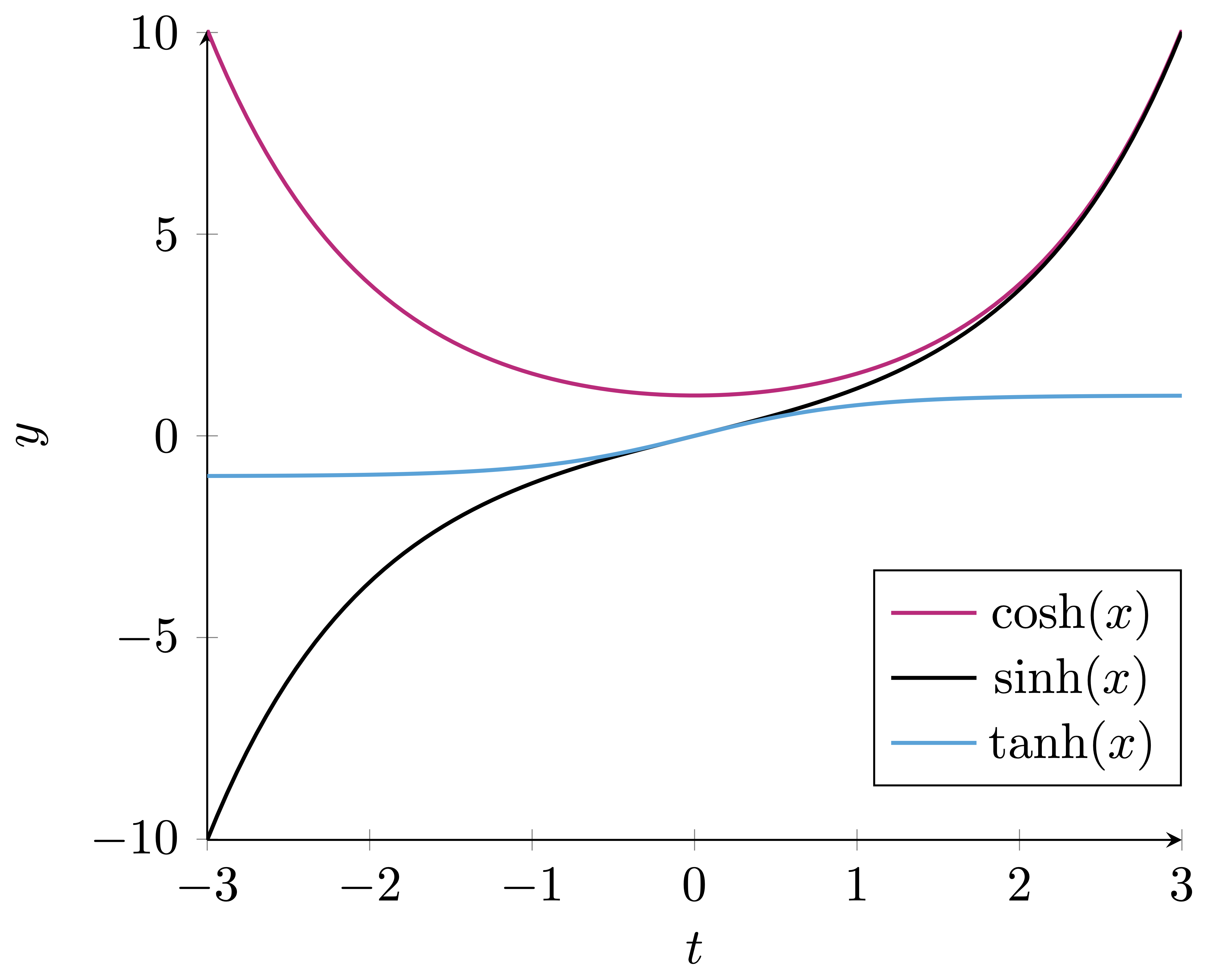
For a plot $\cosh ,\sinh ,\tanh$ see Figure 2.1 below. The properties of the hyperbolic functions which are of interest to us are:

1. Identities: $$\begin{array}{rl}& \cosh (t)+\sinh (t)=e^t\\ & \cosh (t)-\sinh (t)=e^{-t}\\ & {\cosh }^2(t)-{\sinh }^2(t)=1\\ & {\mathrm{sech}}^2(t)-{\tanh }^2(t)=1\end{array}$$

2. Derivatives: $$\begin{array}{rl}\frac{d}{dt}[\sinh (t)]& =\cosh (t)\\ \frac{d}{dt}[\cosh (t)]& =\sinh (t)\\ \frac{d}{dt}[\tanh (t)]& =1-{\tanh }^2(t)=-{\mathrm{csch}}^2(t)\end{array}$$

3. Integrals: $$\begin{array}{rl}{\int }_{t_0}^t\sinh (u)du& =\cosh (t)-\cosh (t_0)\\ {\int }_{t_0}^t\cosh (u)du& =\sinh (t)-\sinh (t_0)\\ {\int }_{t_0}^t\tanh (u)du& =\log (\cosh (t))-\log (\cosh (t_0))\end{array}$$

Figure 2.1: Plot of $\cosh ,\sinh ,\tanh$.

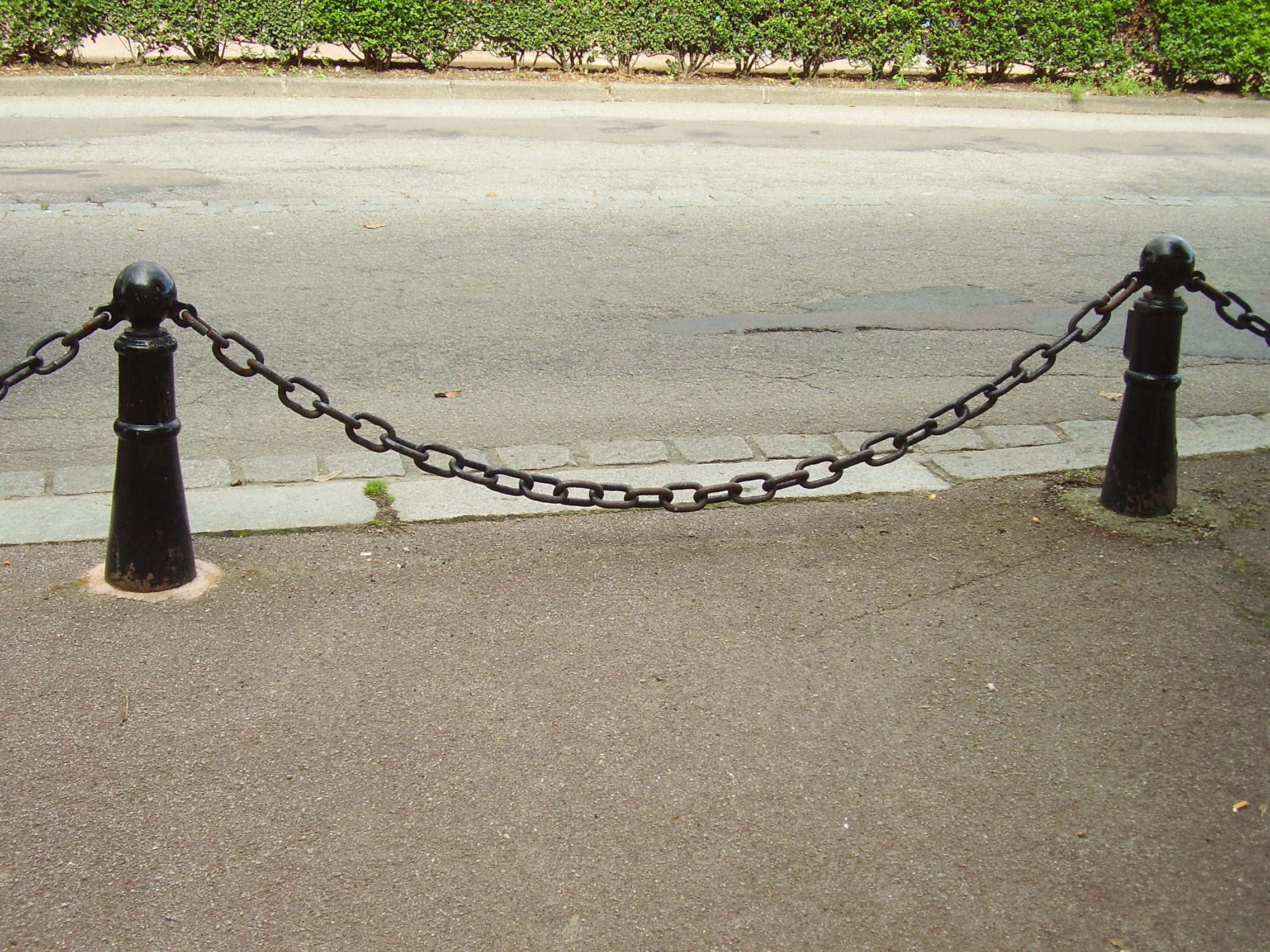
Example 7: The Catenary

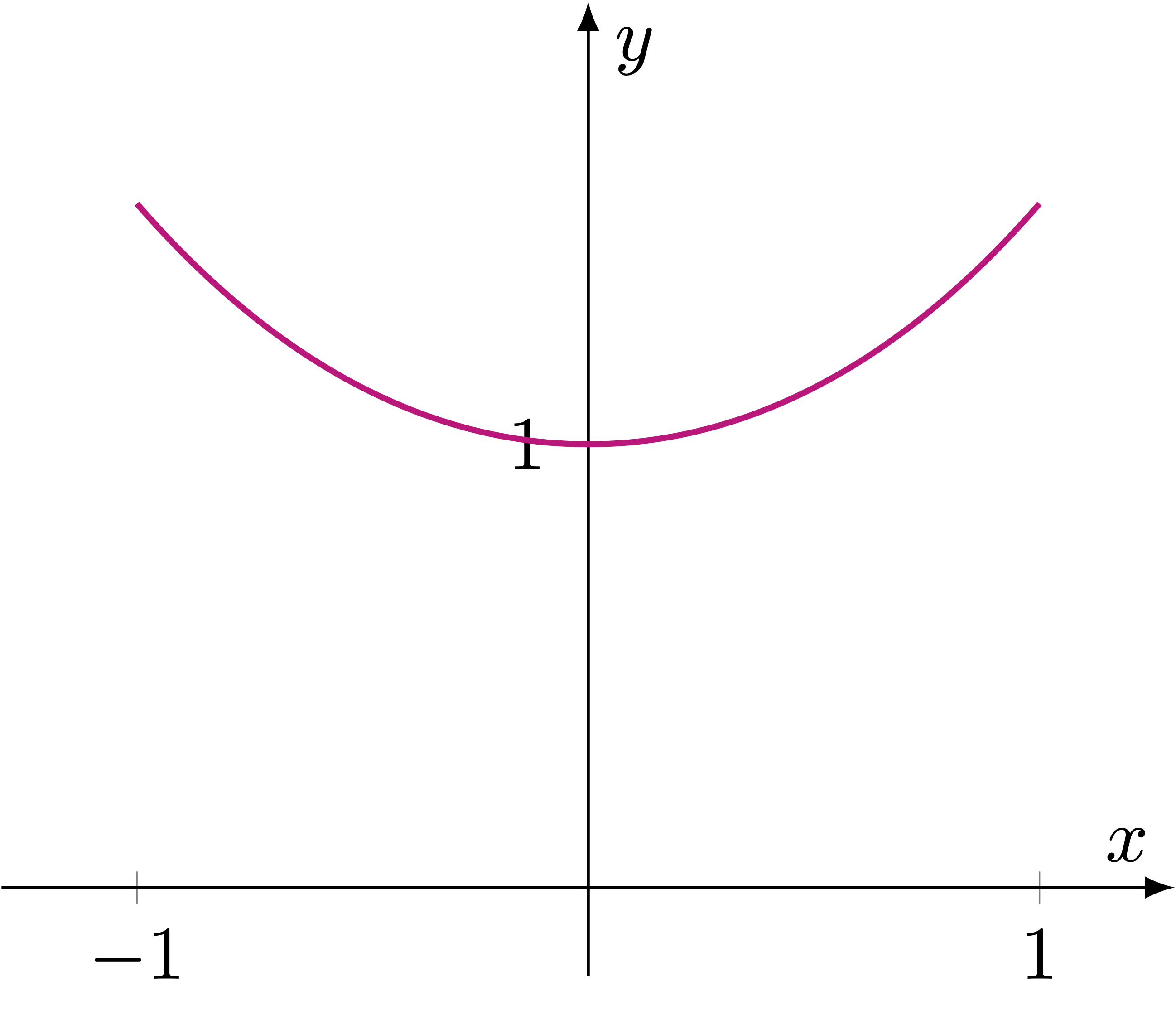
The catenary is the shape of a heavy chain suspended at its ends. The chain is only subjected to gravity, see Figure 2.2. This shape looks similar to a parabola, but it is not a parabola. This was first noted by Galilei, see this Wikipedia page. The profile of the hanging chain can be obtained via a minimization problem, and one can show it is of the form $$\gamma \gamma (t)=(t,\cosh (t)),t\in \mathbb{R}.$$ See Figure 2.3 for a plot of $\gamma \gamma$. Let us check if $\gamma \gamma$ is regular. We have $$\dot{\gamma \gamma }(t)=(1,\sinh (t))$$ so that $${\Vert \dot{\gamma \gamma }\Vert }^2=1+{\sinh }^2(t)={\cosh }^2(t)⟹\Vert \dot{\gamma \gamma }\Vert =\cosh (t).$$ Note that $$\cosh (t)\ge 1$$ showing that $\gamma \gamma$ is regular. However $$\Vert \dot{\gamma \gamma }(1)\Vert =\cosh (1)=\frac{e+e^{-1}}{2}\approx 1.54,$$ proving that $\gamma \gamma$ is not unit speed. Let us then compute the arc length of $\gamma \gamma$ starting at $t_0=0$ $$s(t)={\int }_0^t\Vert \dot{\gamma \gamma }(u)\Vert du={\int }_0^t\cosh (u)du=\sinh (t)$$ since $\sinh (0)=0$. We need to invert $s$. We have $$s=\sinh (t)⟺s=\frac{e^t-e^{-t}}{2}⟺e^{2t}-2s{e}^t-1=0,$$ where the last equation was obtained multuplying both sides by $e^t$. Now we substitute $$y=e^t$$ and obtain $$e^{2t}-2s{e}^t-1=0⟺y^2-2sy-1=0⟺y=s\pm \sqrt{1+s^2}.$$ Recalling that $y=e^t$, we only consider the positive solution, and obtain that $$e^t=s+\sqrt{1+s^2}⟹t=\log (s+\sqrt{1+s^2}).$$ We have proven that the inverse of the arc length $s(t)$ is $$\psi (t):=s^{-1}(t)=\log (t+\sqrt{1+t^2}).$$ Therefore $$\widetilde{\gamma \gamma }(t):=\gamma \gamma (\psi (t))$$ is a unit speed reparametrization of $\gamma \gamma$. Substituting $\psi$ and using the definition of $\gamma \gamma$ we have $$\widetilde{\gamma \gamma }(t)=(\log (t+\sqrt{1+t^2}),\sqrt{1+t^2}).$$ We can now compute the curvature. We have: $$\begin{array}{rl}\dot{\widetilde{\gamma \gamma }}(t)& =(\frac{1}{\sqrt{1+t^2}},\frac{t}{\sqrt{1+t^2}})\\ \ddot{\widetilde{\gamma \gamma }}(t)& =(-\frac{t}{(1+t^2{)}^{3/2}},\frac{1}{(1+t^2{)}^{3/2}})\end{array}$$ Moreover $${\Vert \ddot{\widetilde{\gamma \gamma }}(t)\Vert }^2=\frac{t^2}{(1+t^2{)}^3}+\frac{1}{(1+t^2{)}^3}=\frac{1}{(1+t^2{)}^2}.$$ Therefore the curvature is $$\kappa (t)=\Vert \ddot{\widetilde{\gamma \gamma }}(t)\Vert =\frac{1}{1+t^2}.$$

Figure 2.2: The catenary is the shape of a heavy chain suspended at its ends. Image from Wikipedia.

Figure 2.3: Plot of the catenary curve $\gamma \gamma (t)=(t,\cosh (t))$.

2.2 Vector product in ${\mathbb{R}}^3$

The discussion in this section follows (do Carmo 2017). We start by defining orientation for a vector space.

Definition 8: Same orientation

Consider two ordered basis of ${\mathbb{R}}^3$ $$B=({\mathbf{b}}_1,{\mathbf{b}}_2,{\mathbf{b}}_3),\tilde{B}=({\tilde{\mathbf{b}}}_1,{\tilde{\mathbf{b}}}_2,{\tilde{\mathbf{b}}}_3).$$ We say that $B$ and $\tilde{B}$ have the same orientation if the matrix of change of basis has positive determinant.

When two basis $B$ and $\tilde{B}$ have the same orientation, we write $$\mathbf{b}\sim \tilde{\mathbf{b}}.$$ The above is clearly an equivalence relation on the set of ordered basis. Therefore the set of ordered basis of ${\mathbb{R}}^3$ can be decomposed into equivalence classes. Since the determinant of the matrix of change of basis can only be positive or negative, there are only two equivalence classes.

Definition 9: Orientation

The two equivalence classes determined by $\sim$ on the set of ordered basis are called orientations.

Definition 10: Positive orientation

Consider the standard basis of ${\mathbb{R}}^3$ $$E=({\mathbf{e}}_1,{\mathbf{e}}_2,{\mathbf{e}}_3)$$ where we set $${\mathbf{e}}_1=(1,0,0),{\mathbf{e}}_2=(0,1,0),{\mathbf{e}}_3=(0,0,1).$$ Then:

• The orientation corresponding to $E$ is called positive orientation of ${\mathbb{R}}^3$.
• The orientation corresponding to the other equivalence class is called negative orientation of ${\mathbb{R}}^3$.

For a basis $B$ of ${\mathbb{R}}^3$ we say that:

• $B$ is a positive basis if it belongs to the class of $e$.
• $B$ is a negative basis if it does not belong to the class of $e$.

Example 11

Since we are dealing with ordered basis, the order in which vectors appear is fundamental. For example, we defined the equivalence class of $$E=({\mathbf{e}}_1,{\mathbf{e}}_2,{\mathbf{e}}_3),$$ to be the positive orientation of ${\mathbb{R}}^3$. In particular $e$ is a positive basis.
Consider instead $$\tilde{E}=({\mathbf{e}}_2,{\mathbf{e}}_1,{\mathbf{e}}_3).$$ The matrix of change of variables between $\tilde{E}$ and $E$ is $$({\mathbf{e}}_2|{\mathbf{e}}_1|{\mathbf{e}}_3)=\left(\begin{array}{ccc}0& 1& 0\\ 1& 0& 0\\ 0& 0& 1\end{array}\right)$$ and the latter has negative determinant. Thus $\tilde{E}$ does not belong to the class of $E$, and is therefore a negative basis.

We are now ready to define the vector product in ${\mathbb{R}}^3$.

Definition 12: Vector product in ${\mathbb{R}}^3$

Let $\mathbf{u},\mathbf{v}\in {\mathbb{R}}^3$. The vector product of $\mathbf{u}$ and $\mathbf{v}$ is the unique vector $$\mathbf{u}\times \mathbf{v}\in {\mathbb{R}}^3$$ which satisfies the property: $$\begin{array}{}\text{(2.5)}& (\mathbf{u}\times \mathbf{v})\cdot \mathbf{w}=\left|\begin{array}{ccc}{u}_1& u_2& u_3\\ v_1& v_2& v_3\\ w_1& w_2& w_3\end{array}\right|,\mathrm{\forall }\mathbf{w}\in {\mathbb{R}}^3.\end{array}$$ Here $|a_{ij}|$ denotes the determinant of the matrix $(a_{ij})$, and $$\mathbf{u}=\sum _{i=1}^3{u}_i{\mathbf{e}}_i,\mathbf{v}=\sum _{i=1}^3{v}_i{\mathbf{e}}_i,\mathbf{w}=\sum _{i=1}^3{w}_i{\mathbf{e}}_i,$$ with $({\mathbf{e}}_1,{\mathbf{e}}_2,{\mathbf{e}}_3)$ standard basis of ${\mathbb{R}}^3$.

The following proposition gives an explicit formula for computing $\mathbf{u}\times \mathbf{v}$.

Proposition 13

Let $\mathbf{u},\mathbf{v}\in {\mathbb{R}}^3$. Then $$\begin{array}{}\text{(2.6)}& \mathbf{u}\times \mathbf{v}=\left|\begin{array}{cc}{u}_2& u_3\\ v_2& v_3\end{array}\right|{\mathbf{e}}_1-\left|\begin{array}{cc}{u}_1& u_3\\ v_1& v_3\end{array}\right|{\mathbf{e}}_2+\left|\begin{array}{cc}{u}_1& u_2\\ v_1& v_2\end{array}\right|{\mathbf{e}}_3.\end{array}$$

Proof

Denote by $(\mathbf{u}\times \mathbf{v}{)}_i$ the $i$-th component of $\mathbf{u}\times \mathbf{v}$ with respect to the standard basis, that is, $$\mathbf{u}\times \mathbf{v}=\sum _{i=1}^3(\mathbf{u}\times \mathbf{v}{)}_i{\mathbf{e}}_i.$$ We can use (2.5) with $\mathbf{w}={\mathbf{e}}_1$ to obtain $$(\mathbf{u}\times \mathbf{v})\cdot {\mathbf{e}}_1=\left|\begin{array}{ccc}{u}_1& u_2& u_3\\ v_1& v_2& v_3\\ 1& 0& 0\end{array}\right|=\left|\begin{array}{cc}{u}_2& u_3\\ v_2& v_3\end{array}\right|$$ where we used the Laplace expansion for computing the determinant of the $3\times 3$ matrix. As the standard basis is orthonormal, by bilinearity of the scalar product we get $$(\mathbf{u}\times \mathbf{v})\cdot {\mathbf{e}}_1=\sum _{i=1}^3(\mathbf{u}\times \mathbf{v}{)}_i{\mathbf{e}}_i\cdot {\mathbf{e}}_1=(\mathbf{u}\times \mathbf{v}{)}_i.$$ Therefore we have shown $$(\mathbf{u}\times \mathbf{v}{)}_1=\left|\begin{array}{cc}{u}_2& u_3\\ v_2& v_3\end{array}\right|.$$ Similarly we obtain $$(\mathbf{u}\times \mathbf{v}{)}_2=\left|\begin{array}{ccc}{u}_1& u_2& u_3\\ v_1& v_2& v_3\\ 0& 1& 0\end{array}\right|=-\left|\begin{array}{cc}{u}_1& u_3\\ v_1& v_3\end{array}\right|$$ and $$(\mathbf{u}\times \mathbf{v}{)}_3=\left|\begin{array}{ccc}{u}_1& u_2& u_3\\ v_1& v_2& v_3\\ 0& 0& 1\end{array}\right|=\left|\begin{array}{cc}{u}_1& u_2\\ v_1& v_2\end{array}\right|,$$ from which we conclude.

Sometimes we will denote formula (2.6) by $$\mathbf{u}\times \mathbf{v}=\left|\begin{array}{ccc}\mathbf{i}& \mathbf{j}& \mathbf{k}\\ u_1& u_2& u_2\\ v_1& v_2& v_3\end{array}\right|.$$

Let us collect some crucial properties of the vector product.

Proposition 14

The vector product in ${\mathbb{R}}^3$ satisfies the following properties: For all $\mathbf{u},\mathbf{v}\in {\mathbb{R}}^3$

1. $\mathbf{u}\times \mathbf{v}=-\mathbf{v}\times \mathbf{u}$
2. $\mathbf{u}\times \mathbf{v}=00$ if and only if $\mathbf{u}$ and $\mathbf{v}$ are linearly dependent
3. $(\mathbf{u}\times \mathbf{v})\cdot \mathbf{u}=0$, $(\mathbf{u}\times \mathbf{v})\cdot \mathbf{v}=0$
4. For all $\mathbf{w}\in {\mathbb{R}}^3$, $a,b\in \mathbb{R}$ $$(a\mathbf{u}+b\mathbf{w})\times \mathbf{v}=a\mathbf{u}\times \mathbf{v}+b\mathbf{w}\times \mathbf{w}$$

The proof, which is based on the properties of determinants, is omitted.

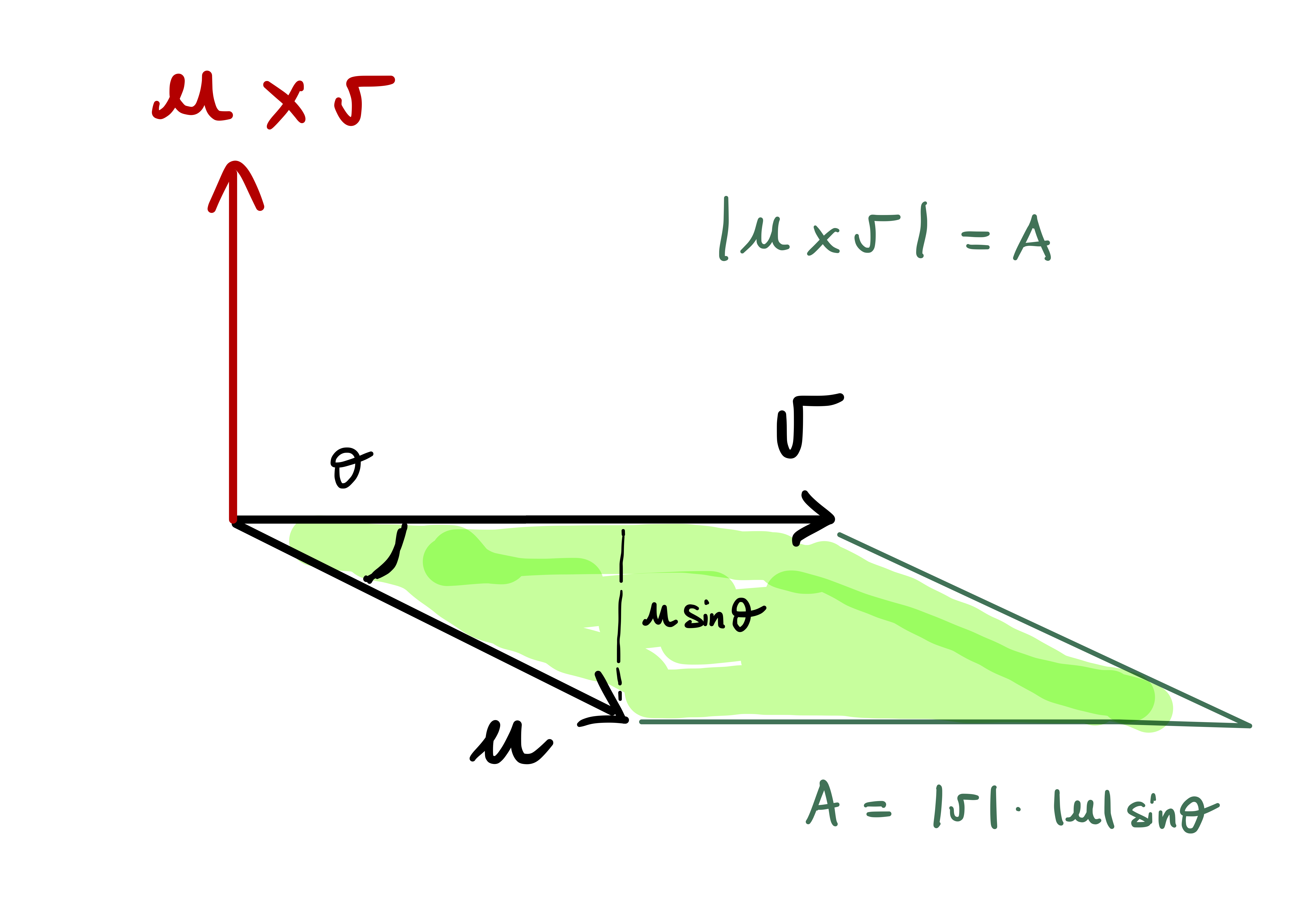
Remark 15: Geometric interpretation of vector product

Let $\mathbf{u},\mathbf{v}\in {\mathbb{R}}^3$ be linearly independent. We make some observations:

1. Property 3 in Proposition 14 says that $$(\mathbf{u}\times \mathbf{v})\cdot \mathbf{u}=0,(\mathbf{u}\times \mathbf{v})\cdot \mathbf{v}=0.$$ Therefore $\mathbf{u}\times \mathbf{v}$ is orthogonal to both $\mathbf{u}$ and $\mathbf{v}$.

2. In particular $\mathbf{u}\times \mathbf{v}$ is orthogonal to the plane generated by $\mathbf{u}$ and $\mathbf{v}$.

3. Since $\mathbf{u}$ and $\mathbf{v}$ are linearly independent, Property 2 in Proposition 14 says that $$\mathbf{u}\times \mathbf{v}\ne 00$$

4. Therefore we have $$(\mathbf{u}\times \mathbf{v})\cdot (\mathbf{u}\times \mathbf{v})={\Vert \mathbf{u}\times \mathbf{v}\Vert }^2>0$$

5. On the other hand, using the definition of $\mathbf{u}\times \mathbf{v}$ with $\mathbf{w}=\mathbf{v}\times \mathbf{w}$ yields $$(\mathbf{u}\times \mathbf{v})\cdot (\mathbf{u}\times \mathbf{v})=\left|\begin{array}{ccc}{u}_1& u_2& u_3\\ v_1& v_2& v_3\\ (\mathbf{u}\times \mathbf{v}{)}_1& (\mathbf{u}\times \mathbf{v}{)}_2& (\mathbf{u}\times \mathbf{v}{)}_3\end{array}\right|$$

6. Therefore the determinant of the matrix $$(\mathbf{u}|\mathbf{v}|\mathbf{u}\times \mathbf{v})$$ is positive. This shows that $$(\mathbf{u},\mathbf{v},\mathbf{u}\times \mathbf{v})$$ is a positive basis of ${\mathbb{R}}^3$.

7. For all $\mathbf{u},\mathbf{v},\mathbf{x},\mathbf{y}\in {\mathbb{R}}^3$ it holds $$\begin{array}{}\text{(2.7)}& (\mathbf{u}\times \mathbf{v})\cdot (\mathbf{x}\times \mathbf{y})=\left|\begin{array}{cc}\mathbf{u}\cdot \mathbf{x}& \mathbf{v}\cdot \mathbf{x}\\ \mathbf{u}\cdot \mathbf{y}& \mathbf{v}\cdot \mathbf{y}\end{array}\right|.\end{array}$$ Indeed, one can check that the above formula holds for the standard vectors ${\mathbf{e}}_i$, and thus the general formula follows by linearity.

8. Using (2.7) we get $$\begin{array}{rl}{\Vert \mathbf{u}\times \mathbf{v}\Vert }^2& =(\mathbf{u}\times \mathbf{v})\cdot (\mathbf{u}\times \mathbf{v})=\left|\begin{array}{cc}\mathbf{u}\cdot \mathbf{u}& \mathbf{v}\cdot \mathbf{u}\\ \mathbf{u}\cdot \mathbf{v}& \mathbf{v}\cdot \mathbf{v}\end{array}\right|\\ & ={\Vert \mathbf{u}\Vert }^2{\Vert \mathbf{v}\Vert }^2-|\mathbf{u}\cdot \mathbf{v}{|}^2\\ & ={\Vert \mathbf{u}\Vert }^2{\Vert \mathbf{v}\Vert }^2-{\Vert \mathbf{u}\Vert }^2{\Vert \mathbf{v}\Vert }^2{\cos }^2(\theta )\\ & ={\Vert \mathbf{u}\Vert }^2{\Vert \mathbf{v}\Vert }^2(1-{\cos }^2(\theta ))\\ & ={\Vert \mathbf{u}\Vert }^2{\Vert \mathbf{v}\Vert }^2{\sin }^2(\theta )\\ & =A^2\end{array}$$ where $A$ is the area of the parallelogram with sides $\mathbf{u}$ and $\mathbf{v}$.

For $\mathbf{u},\mathbf{v}$ linearly independent, $\mathbf{u}\times \mathbf{v}$ is orthogonal to the plane generated by $\mathbf{u},\mathbf{v}$. Moreover $|\mathbf{u}\times \mathbf{v}|$ is the area of the parallelogram with sides $\mathbf{u},\mathbf{v}$, and $(\mathbf{u},\mathbf{v},\mathbf{u}\times \mathbf{v})$ is a positive basis of ${\mathbb{R}}^3$

Let us summarize the above remark.

Remark 16: Summary: Properties of $\mathbf{u}\times \mathbf{v}$

Let $\mathbf{u},\mathbf{v}\in {\mathbb{R}}^3$ be linearly independent. Then

• $\mathbf{u}\times \mathbf{v}$ is orthogonal to the plane spanned by $\mathbf{u},\mathbf{v}$
• $\Vert \mathbf{u}\times \mathbf{v}\Vert$ is equal to the area of the parallelogram with sides $\mathbf{u},\mathbf{v}$
• $\mathbf{u}\times \mathbf{v}$ is such that $$(\mathbf{u},\mathbf{v},\mathbf{u}\times \mathbf{v})$$ is a positive basis of ${\mathbb{R}}^3$.

We conclude with noting that the cross product is not associative, and with a useful proposition for differentiating the cross product of curves in ${\mathbb{R}}^3$.

Proposition 17

The vector product is not associative. In particular, for all $\mathbf{u},\mathbf{v},\mathbf{w}\in {\mathbb{R}}^3$ it holds: $$\begin{array}{}\text{(2.8)}& (\mathbf{u}\times \mathbf{v})\times \mathbf{w}=(\mathbf{u}\cdot \mathbf{w})\mathbf{v}-(\mathbf{v}\cdot \mathbf{w})\mathbf{u}.\end{array}$$

The proof is omitted. It follows by observing that both sides of (2.8) are linear in $\mathbf{u},\mathbf{v},\mathbf{w}$. Therefore it is sufficient to verify (2.8) for the standard basis vectors ${\mathbf{e}}_i$. This is left as an exercise.

Proposition 18

Suppose $\gamma \gamma ,\eta \eta :(a,b)\to {\mathbb{R}}^3$ are parametrized curves. Then the curve $$\gamma \gamma \times \eta \eta :(a,b)\to {\mathbb{R}}^3$$ is smooth, and $$\begin{array}{}\text{(2.9)}& \frac{d}{dt}(\gamma \gamma \times \eta \eta )=\dot{\gamma \gamma }\times \eta \eta +\gamma \gamma \times \dot{\eta \eta }.\end{array}$$

The proof is omitted. It follows immediately from formula (2.6).

2.3 Curvature formula in ${\mathbb{R}}^3$

Given a unit speed curve $$\gamma \gamma :(a,b)\to {\mathbb{R}}^n$$ we defined its curvature as $$\kappa (t)=\Vert \ddot{\gamma \gamma }(t)\Vert .$$ If $\gamma \gamma$ is not unit speed then the curvature is not defined. However, when $\gamma \gamma$ is regular, then we can find a unit-speed reparametrization $\widetilde{\gamma \gamma }$ of $\gamma \gamma$, and compute $\kappa$ as $$\kappa (t)=\Vert \ddot{\widetilde{\gamma \gamma }}(t)\Vert .$$ If $\gamma \gamma$ is a regular curve in ${\mathbb{R}}^3$, there is a way to compute $\kappa$ without passing through $\widetilde{\gamma \gamma }$. The formula for computing $\kappa$ is as follows.

Proposition 19: Curvature formula

Let $\gamma \gamma :(a,b)\to {\mathbb{R}}^3$ be a regular curve. The curvature $\kappa (t)$ of $\gamma \gamma$ at $\gamma \gamma (t)$ is given by $$\begin{array}{}\text{(2.10)}& \kappa (t)=\frac{\Vert \dot{\gamma \gamma }\times \ddot{\gamma \gamma }\Vert }{{\Vert \dot{\gamma \gamma }\Vert }^3}.\end{array}$$

We delay the proof of the above Proposition, as this will get easier when the Frenet frame is introduced. For a proof which does not make use of the Frenet frame, see the proof of Proposition 2.1.2 in (Pressley 2010).

For now we use (2.10) the above proposition to compute the curvature on specific curves.

Example 20

Consider the straight line $$\gamma \gamma (t)=\mathbf{a}+t\mathbf{v}$$ for some $\mathbf{a},\mathbf{v}\in {\mathbb{R}}^3$ fixed, with $\mathbf{v}\ne 00$. Then $$\dot{\gamma \gamma }(t)=\mathbf{v},\ddot{\gamma \gamma }(t)=00.$$ Therefore $$\Vert \dot{\gamma \gamma }(t)\Vert =\Vert \mathbf{v}\Vert \ne 0$$ showing that $\gamma \gamma$ is regular. We have $$\dot{\gamma \gamma }\times \ddot{\gamma \gamma }=\mathbf{v}\times 00=00.$$ Therefore the curvature is $$\kappa =\frac{\Vert \dot{\gamma \gamma }\times \ddot{\gamma \gamma }\Vert }{{\Vert \dot{\gamma \gamma }\Vert }^3}=0,$$ as expected.

Example 21

Consider the Helix of radius $R>0$ and rise $H>0$ $$\gamma \gamma (t)=(R\cos (t),R\sin (t),Ht),t\in \mathbb{R}.$$ Then $$\begin{array}{rl}\dot{\gamma \gamma }(t)& =(-R\sin (t),R\cos (t),H)\\ \ddot{\gamma \gamma }(t)& =(-R\cos (t),-R\sin (t),0)\end{array}$$ From this we deduce that $$\Vert \dot{\gamma \gamma }(t)\Vert =\sqrt{R^2+H^2},$$ showing that $\gamma \gamma$ is regular. Finally $$\begin{array}{rl}\dot{\gamma \gamma }\times \ddot{\gamma \gamma }& =\left|\begin{array}{cc}{\dot{\gamma }}_2& {\dot{\gamma }}_3\\ {\ddot{\gamma }}_2& {\ddot{\gamma }}_3\end{array}\right|{\mathbf{e}}_1-\left|\begin{array}{cc}{\dot{\gamma }}_1& {\dot{\gamma }}_3\\ {\ddot{\gamma }}_1& {\ddot{\gamma }}_3\end{array}\right|{\mathbf{e}}_2+\left|\begin{array}{cc}{\dot{\gamma }}_1& {\dot{\gamma }}_2\\ {\ddot{\gamma }}_1& {\ddot{\gamma }}_2\end{array}\right|{\mathbf{e}}_3\\ & =\left|\begin{array}{cc}R\cos (t)& H\\ -R\sin (t)& 0\end{array}\right|{\mathbf{e}}_1-\left|\begin{array}{cc}-R\sin (t)& H\\ -R\cos (t)& 0\end{array}\right|{\mathbf{e}}_2+\left|\begin{array}{cc}-R\sin (t)& R\cos (t)\\ -R\cos (t)& -R\sin (t)\end{array}\right|{\mathbf{e}}_3\\ & =(RH\sin (t),-RH\cos (t),R^2{\cos }^2(t)+R^2{\sin }^2(t))\\ & =(RH\sin (t),-RH\cos (t),R^2)\end{array}$$ and therefore $$\Vert \dot{\gamma \gamma }\times \ddot{\gamma \gamma }\Vert =R\sqrt{R^2+H^2}.$$ By the general formula we have $$\kappa =\frac{\Vert \dot{\gamma \gamma }\times \ddot{\gamma \gamma }\Vert }{{\Vert \dot{\gamma \gamma }\Vert }^3}=\frac{R(R^2+H^2{)}^{\frac{1}{2}}}{(R^2+H^2{)}^{\frac{3}{2}}}=\frac{R}{R^2+H^2}$$

We notice the following:

• If $H=0$ then the Helix is just a circle of radius $R$. In this case the curvature is $$\kappa =\frac{1}{R}$$ which agrees with the curvature computed for the circle of radius $R$.

• If $R=0$ then the Helix is just parametrizing the $z$-axis. In this case the curvature is $$\kappa =0,$$ which agrees with the curvature of a straight line.

2.4 Signed curvature of plane curves

In this section we assume to have plane curves, that is, curves with values in ${\mathbb{R}}^2$. In this case we can give a geometric interpretation for the sign of the curvature. This cannot be done in higher dimension.

Definition 22

Let $\gamma \gamma :(a,b)\to {\mathbb{R}}^2$ be unit speed. We define the signed unit normal to $\gamma \gamma$ at $\gamma \gamma (t)$ as the unit vector $\mathbf{n}(t)$ obtained by rotating $\dot{\gamma \gamma }(t)$ anti-clockwise by an angle of $\pi /2$.

Definition 23

Let $\gamma \gamma :(a,b)\to {\mathbb{R}}^2$ be unit speed. The signed curvature of $\gamma \gamma$ at $\gamma \gamma (t)$ is the scalar ${\kappa }_s(t)$ such that $$\ddot{\gamma \gamma }(t)=k_s(t)\mathbf{n}(t)$$

Remark 24

Notice that since $\mathbf{n}$ is a unit vector and $\gamma \gamma$ is unit speed, then $$|{\kappa }_s(t)|=\Vert \ddot{\gamma \gamma }(t)\Vert =\kappa (t).$$ Thus the signed curvature is related to the curvature by $${\kappa }_s(t)=\pm \kappa (t).$$

Remark 25

It can be shown that the signed curvature is the rate at which the tangent vector $\dot{\gamma \gamma }$ of the curve $\gamma \gamma$ rotates. The signed curvature is:

• positive if $\dot{\gamma \gamma }$ is rotating anti-clockwise
• negative if $\dot{\gamma \gamma }$ is rotating clockwise

In other words,

• $k_s>0$ means the curve is turning left,
• $k_s<0$ means the curve is turning right.

A rigorous justification of the above statement is found in Proposition 2.2.3 in (Pressley 2010).

For curves which are not unit speed, we define the signed curvature as the signed curvature of the unit speed reparametrization.

Definition 26

Let $\gamma \gamma :(a,b)\to {\mathbb{R}}^2$ be regular and let $\widetilde{\gamma \gamma }$ be a unit speed reparametrization of $\gamma \gamma$. The signed curvature of $\gamma \gamma$ at $\gamma \gamma (t)$ is the scalar ${\kappa }_s(t)$ such that $$\ddot{\widetilde{\gamma \gamma }}(t)=k_s(t)\mathbf{n}(t),$$ where $\mathbf{n}(t)$ is the unit vector obtained by rotating $\dot{\widetilde{\gamma \gamma }}(t)$ anti-clockwise by an angle $\pi /2$.

The signed curvature completely characterizes plane curves, in the sense of the following theorem.

Theorem 27: Characterization of plane curves

Let $\varphi :\mathbb{R}\to \mathbb{R}$ be smooth. Then:

1. There exists a unit speed curve $\gamma \gamma :\mathbb{R}\to {\mathbb{R}}^2$ such that its signed curvature ${\kappa }_s$ satisfies $${\kappa }_s(t)=\varphi (t),\mathrm{\forall }t\in \mathbb{R}.$$

2. Suppose that $\widetilde{\gamma \gamma }:\mathbb{R}\to {\mathbb{R}}^2$ is a unit speed curve such that its signed curvature ${\tilde{\kappa }}_s$ satisfies $${\tilde{\kappa }}_s(t)=\varphi (t),\mathrm{\forall }t\in \mathbb{R}.$$ Then $$\widetilde{\gamma \gamma }=\gamma \gamma$$ up to rotations and translations.

We do not prove the above theorem. For a proof, see Theorem 2.2.6 in (Pressley 2010).

2.5 Space curves

In this section we deal with space curves, that is, curves with values in ${\mathbb{R}}^3$. There are several issues compare to the plane case:

• A 3D counterpart of the signed curvature does not exist, since there is no notion of turning left or turning right.

• We have seen in the previous section that the signed curvature completely characterizes plane curves. In 3D however curvature is not enough to characterize curves: there exist $\gamma \gamma$ and $\eta \eta$ space curves such that $${\kappa }^{\gamma \gamma }={\kappa }^{\eta \eta },\gamma \gamma \ne \eta \eta ,$$ that is, $\gamma \gamma$ and $\eta \eta$ have same curvature but are different curves.

Example 28

Let $\gamma \gamma$ be a circle of radius $R>0$ $$\gamma \gamma (t)=(R\cos (t),R\sin (t),0),$$ and $\eta \eta$ be a helix of radius $S>0$ and rise $H>0$ $$\eta \eta (t)=(S\cos (t),S\sin (t),Ht).$$ We have computed that $${\kappa }^{\gamma \gamma }=\frac{1}{R},{\kappa }^{\eta \eta }=\frac{S}{S^2+H^2}.$$ If we now choose $R=2$ and we impose that ${\kappa }^{\gamma \gamma }={\kappa }^{\eta \eta }$ we get $$\frac{1}{R}=\frac{S}{S^2+H^2}⟹H^2=2S-S^2$$ Therefore choosing $S=1$ and $H=1$ yields $${\kappa }^{\gamma \gamma }={\kappa }^{\eta \eta },\gamma \gamma \ne \eta \eta ..$$

Therefore curvature is not enough for characterizing space curves, and we need a new quantity. As we did with curvature, we start by considering the simpler case of unit speed curves. We will also need to assume that the curvature is never zero.

Definition 29: Principal normal vector

Let $\gamma \gamma :(a,b)\to {\mathbb{R}}^3$ be a unit speed curve with $$\kappa (t)\ne 0,\mathrm{\forall }t\in (a,b).$$ The principal normal vector to $\gamma \gamma$ at $\gamma \gamma (t)$ is $$\mathbf{n}(t):=\frac{1}{\kappa (t)}\ddot{\gamma \gamma }(t).$$

Remark 30

Since for $\gamma \gamma$ unit speed we defined $$\kappa (t):=\Vert \ddot{\gamma \gamma }(t)\Vert ,$$ we have that $$\Vert \mathbf{n}(t)\Vert =1,$$ thus $\mathbf{n}$ is a unit vector. Moreover $\mathbf{n}$ is orthogonal to $\dot{\gamma \gamma }$, that is, $$\dot{\gamma \gamma }\cdot \mathbf{n}=0.$$

This is because $$\dot{\gamma \gamma }\cdot \mathbf{n}=\frac{1}{\kappa }\dot{\gamma \gamma }\cdot \ddot{\gamma \gamma }=0,$$ where the last equality follows from $\dot{\gamma \gamma }\cdot \ddot{\gamma \gamma }=0$, being $\gamma \gamma$ unit speed.

Principal normal vector $\mathbf{n}(t)$ to $\gamma \gamma$ at $\gamma \gamma (t)$.

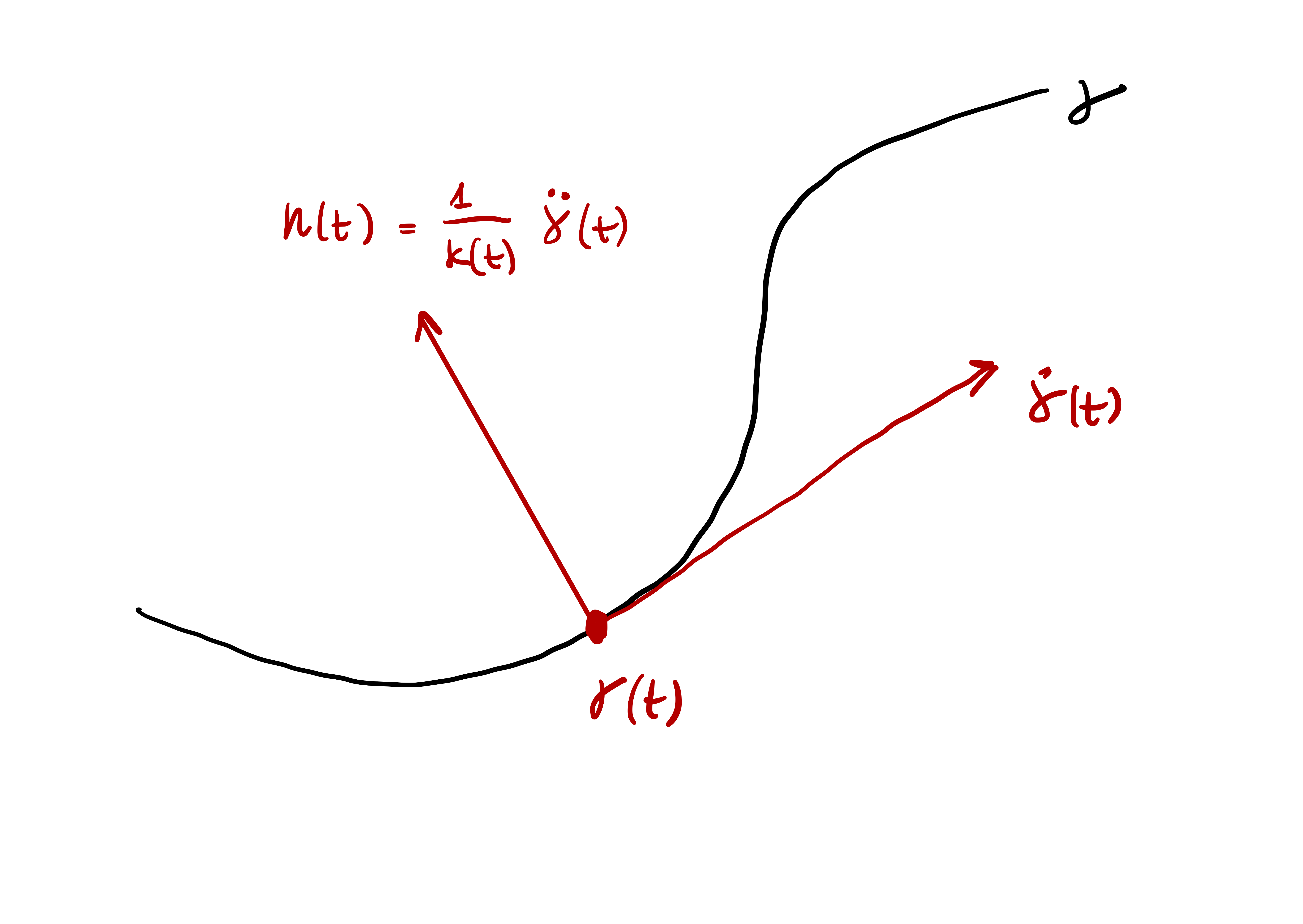
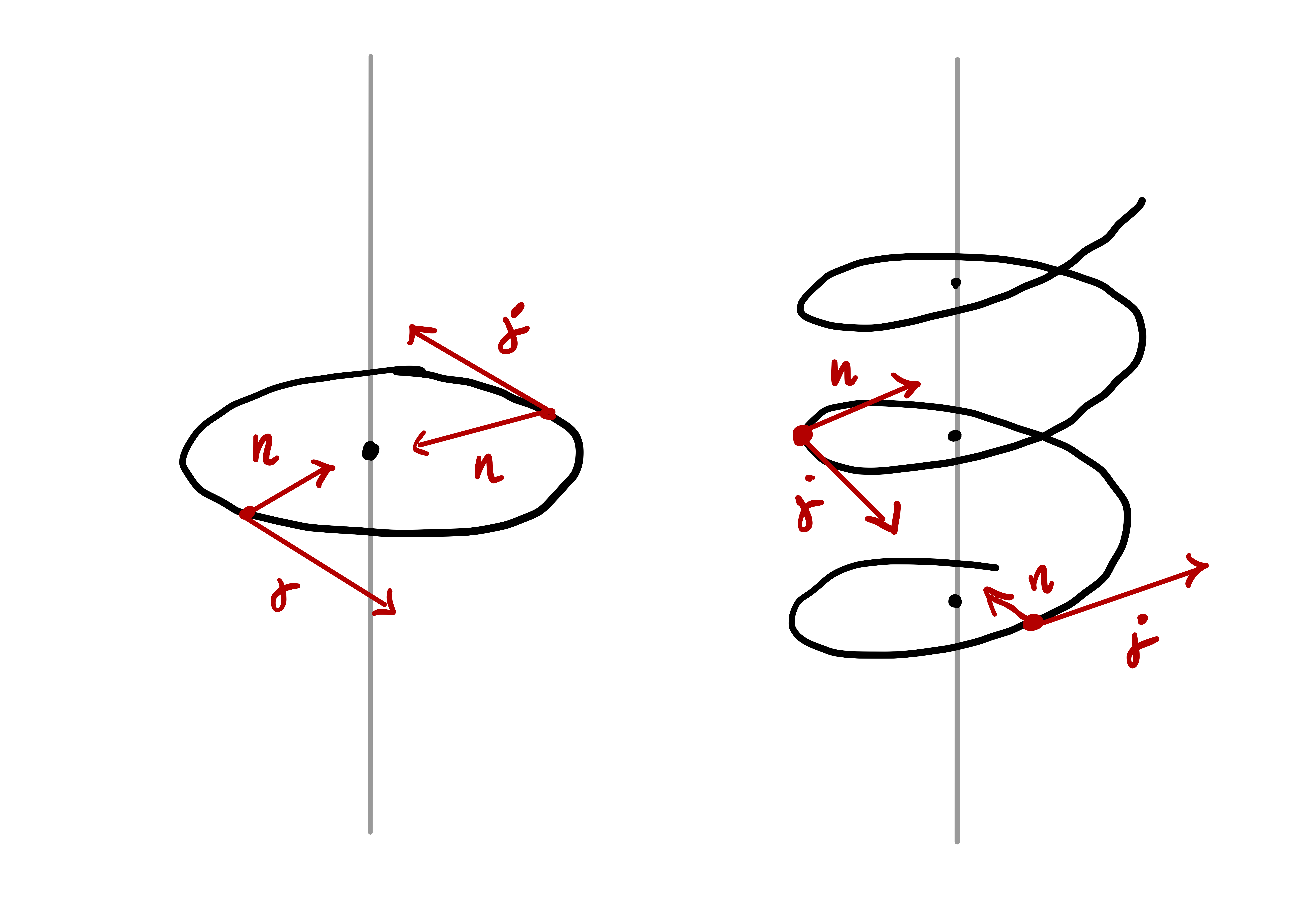
Question 31

Why is the principal normal interesting? Because it can tell the difference beween a plane curve and a space curve. See picture below.

Left: Principal normal to a circle. Note that $\mathbf{n}$ always points towards the origin $00$. Right: Principal normal to a helix. Note that $\mathbf{n}$ points towards the $z$-axis, but never towards the same point.

Definition 32: Binormal vector

Let $\gamma \gamma :(a,b)\to {\mathbb{R}}^3$ be a unit speed curve with $$\kappa (t)\ne 0,\mathrm{\forall }t\in (a,b).$$ The binormal vector to $\gamma \gamma$ at $\gamma \gamma (t)$ is $$\mathbf{b}(t):=\dot{\gamma \gamma }(t)\times \mathbf{n}(t).$$

Definition 33: Orthonormal basis

Let ${\mathbf{v}}_1,{\mathbf{v}}_2,{\mathbf{v}}_3$ be vectors in ${\mathbb{R}}^3$. We say that the triple $$\{{\mathbf{v}}_1,{\mathbf{v}}_2,{\mathbf{v}}_3\}$$ is orthonormal if $$\Vert v_i\Vert =1,v_i\cdot v_j=0,\text{ for }i\ne j.$$

Proposition 34

Let $\gamma \gamma :(a,b)\to {\mathbb{R}}^3$ be a unit speed curve with $$\kappa (t)\ne 0,\mathrm{\forall }t\in (a,b).$$ Then the triple $$B=(\dot{\gamma \gamma }(t),\mathbf{n}(t),\mathbf{b}(t))$$ is a positive orthonormal basis of ${\mathbb{R}}^3$ for all $t\in (a,b)$.

Proof

Since $\gamma \gamma$ is unit speed we have $$\Vert \dot{\gamma \gamma }(t)\Vert \equiv 1.$$ Moreover we have already observed that $$\Vert \mathbf{n}(t)\Vert \equiv 1,\dot{\gamma \gamma }(t)\cdot \mathbf{n}(t)\equiv 0.$$ As $\mathbf{b}$ is defined by $$\mathbf{b}:=\dot{\gamma \gamma }\times \mathbf{n},$$ by the properties of the vector product, see Proposition 14, it follows that $$\mathbf{b}\cdot \dot{\gamma \gamma }=0,\mathbf{b}\cdot \mathbf{n}=0.$$ By the calculation in Remark 15 Point 8, we have that $${\Vert \mathbf{b}\Vert }^2=\parallel \dot{\gamma \gamma }{\parallel }^2\parallel \mathbf{n}{\parallel }^2-|\dot{\gamma \gamma }\cdot \mathbf{n}{|}^2=1.$$ This shows that the vectors $$\{\dot{\gamma \gamma },\mathbf{n},\mathbf{b}\}$$ are orthonormal. By the properties of the vector product, see Remark 15 Point 6, we also know that $$(\dot{\gamma \gamma },\mathbf{n},\mathbf{b})$$ is a positive basis of ${\mathbb{R}}^3$.

Proposition 35

Let $\gamma \gamma :(a,b)\to {\mathbb{R}}^3$ be a unit speed curve with $\kappa \ne 0$. Then $$\begin{array}{}\text{(2.11)}& \mathbf{b}=\dot{\gamma \gamma }\times \mathbf{n},\mathbf{n}=\mathbf{b}\times \dot{\gamma \gamma },\dot{\gamma \gamma }=\mathbf{n}\times \mathbf{b}.\end{array}$$

Proof

The first equality in (2.11) is true by definition of $\mathbf{b}$. For the other $2$ equalities, recall formula (2.8): $$\begin{array}{}\text{(2.12)}& (\mathbf{u}\times \mathbf{v})\times \mathbf{w}=(\mathbf{u}\cdot \mathbf{w})\mathbf{v}-(\mathbf{v}\cdot \mathbf{w})\mathbf{u},\end{array}$$ for all $\mathbf{u},\mathbf{v},\mathbf{w}\in {\mathbb{R}}^3$. Applying the above with $$\mathbf{u}=\dot{\gamma \gamma },\mathbf{v}=\mathbf{n},\mathbf{w}=\dot{\gamma \gamma },$$ yields $$\begin{array}{rl}(\dot{\gamma \gamma }\times \mathbf{n})\times \dot{\gamma \gamma }& =(\dot{\gamma \gamma }\cdot \dot{\gamma \gamma })\mathbf{n}-(\mathbf{n}\cdot \dot{\gamma \gamma })\dot{\gamma \gamma }\\ & ={\Vert \dot{\gamma \gamma }\Vert }^2\mathbf{n}-0\\ & =\mathbf{n},\end{array}$$ where we used that $\dot{\gamma \gamma }$ is a unit vector and $\mathbf{n}\cdot \dot{\gamma \gamma }=0$. Therefore, by definition of $\mathbf{b}$, we have $$\mathbf{b}\times \dot{\gamma \gamma }=(\dot{\gamma \gamma }\times \mathbf{n})\times \dot{\gamma \gamma }=\mathbf{n}$$ showing the second equality in (2.11). For showing the third equality in (2.11), we apply (2.12) with $$\mathbf{u}=\dot{\gamma \gamma },\mathbf{v}=\mathbf{n},\mathbf{w}=\mathbf{n},$$ to get $$\begin{array}{rl}(\dot{\gamma \gamma }\times \mathbf{n})\times \mathbf{n}& =(\dot{\gamma \gamma }\cdot \mathbf{n})\mathbf{n}-(\mathbf{n}\cdot \mathbf{n})\dot{\gamma \gamma }\\ & =0-{\Vert \mathbf{n}\Vert }^2\dot{\gamma \gamma }\\ & =-\dot{\gamma \gamma }\end{array}$$ where we used that $\mathbf{n}$ is a unit vector and $\dot{\gamma \gamma }\cdot \mathbf{n}=0$. Therefore, by definition of $\mathbf{b}$ and anti-commutativity of the vector product, we have $$\mathbf{n}\times \mathbf{b}=-\mathbf{b}\times \mathbf{n}=-(\dot{\gamma \gamma }\times \mathbf{n})\times \mathbf{n}=\dot{\gamma \gamma },$$ showing the last equality in (2.11).

Proposition 36

Let $\gamma \gamma :(a,b)\to {\mathbb{R}}^3$ be a unit speed curve with $\kappa \ne 0$. Then $$\begin{array}{}\text{(2.13)}& \dot{\mathbf{b}}(t)=-\tau (t)\mathbf{n}(t),\end{array}$$ for some $\tau (t)\in \mathbb{R}$.

Proof

By definition of $\mathbf{b}$ and the formula of derivation of the cross product (2.9) we have $$\begin{array}{rl}\dot{\mathbf{b}}& =\frac{d}{dt}(\dot{\gamma \gamma }\times \mathbf{n})\\ & =\ddot{\gamma \gamma }\times \mathbf{n}+\dot{\gamma \gamma }\times \dot{\mathbf{n}}\\ & =\dot{\gamma \gamma }\times \dot{\mathbf{n}},\end{array}$$ where we used that $$\ddot{\gamma \gamma }\times \mathbf{n}=0,$$ since $\mathbf{n}$ is defined by $\mathbf{n}:=\ddot{\gamma \gamma }/\kappa$, and therefore $\mathbf{n}$ and $\ddot{\gamma \gamma }$ are parallel. Hence, we have proven that $$\begin{array}{}\text{(2.14)}& \dot{\mathbf{b}}=\dot{\gamma \gamma }\times \dot{\mathbf{n}}.\end{array}$$ By the properties of the cross product we have that $\mathbf{u}\times \mathbf{v}$ is orthogonal to both $\mathbf{u}$ and $\mathbf{v}$. Thus (2.14) implies that $$\dot{\mathbf{b}}\cdot \dot{\gamma \gamma }=0.$$ Further, observe that $$\frac{d}{dt}(\mathbf{b}\cdot \mathbf{b})=\dot{\mathbf{b}}\cdot \mathbf{b}+\mathbf{b}\cdot \dot{\mathbf{b}}=2\dot{\mathbf{b}}\cdot \mathbf{b}.$$ On the other hand, since $\mathbf{b}$ is a unit vector, we have $$\frac{d}{dt}(\mathbf{b}\cdot \mathbf{b})=\frac{d}{dt}({\Vert \mathbf{b}\Vert }^2)=\frac{d}{dt}(1)=0$$ Therefore $$\dot{\mathbf{b}}\cdot \mathbf{b}=0.$$ To summarize, we have shown that $\dot{\mathbf{b}}$ is orthogonal to $\mathbf{b}$ and $\dot{\gamma \gamma }$. Since $$(\dot{\gamma \gamma },\mathbf{n},\mathbf{b})$$ is an orthonormal basis of ${\mathbb{R}}^3$ we conclude that $\dot{\mathbf{b}}$ is parallel to $\mathbf{n}$. Therefore there exists $\tau (t)\in \mathbb{R}$ such that $$\dot{\mathbf{b}}=-\tau (t)\mathbf{n}(t),$$ concluding the proof.

The scalar $\tau$ in equation (2.13) is called the torsion of $\gamma \gamma$.

Definition 37: Torsion of unit speed curve

Let $\gamma \gamma :(a,b)\to {\mathbb{R}}^3$ be a unit speed curve, with $\kappa \ne 0$. The torsion of $\gamma \gamma$ at $\gamma \gamma (t)$ is the unique scalar $$\tau (t)\in \mathbb{R}$$ such that $$\dot{\mathbf{b}}(t)=-\tau (t)\mathbf{n}(t).$$

Remark 38

In particular the torsion satisfies: $$\tau (t)=-\dot{\mathbf{b}}(t)\cdot \mathbf{n}(t).$$

The above can be immediately obtained by multiplying (2.13) by $\mathbf{n}$. Indeed, $$\dot{\mathbf{b}}=-\tau \mathbf{n}⟹\dot{\mathbf{b}}\cdot \mathbf{n}=-\tau \mathbf{n}\cdot \mathbf{n}=-\tau ,$$ since $\mathbf{n}$ is a unit vector.

Warning

We defined the torsion only for space curves $\gamma \gamma :(a,b)\to {\mathbb{R}}^3$ which are unit speed and have non-vanishing curvature, that is, such that $$\Vert \dot{\gamma \gamma }(t)\Vert =1,\kappa (t)=\Vert \ddot{\gamma \gamma }(t)\Vert \ne 0,$$ for all $t\in (a,b)$.

We can extend the definition of torsion to regular curves $\gamma \gamma$ with non-vanishing curvature. In this case the torsion of $\gamma \gamma$ is defined as the torsion of a unit speed reparametrization of $\gamma \gamma$.

Definition 39

Let $\gamma \gamma :(a,b)\to {\mathbb{R}}^3$ be a regular curve with non-vanishing curvature. Let $\widetilde{\gamma \gamma }$ be a unit speed reparametrization of $\gamma \gamma$, with $$\gamma \gamma =\widetilde{\gamma \gamma }\circ \varphi ,\varphi :(a,b)\to (\tilde{a},\tilde{b}).$$ We define the torsion of $\gamma \gamma$ at $\gamma \gamma (t)$ as $${\tau }^{\gamma \gamma }(t):={\tau }^{\widetilde{\gamma \gamma }}(\varphi (t)),$$ where ${\tau }^{\widetilde{\gamma \gamma }}(s)$ denotes the torsion of $\widetilde{\gamma \gamma }$ at $\widetilde{\gamma \gamma }(s)$.

As usual, it is possible to check that the above definition of torsion does not depend on the choice of unit speed reparametrization $\widetilde{\gamma \gamma }$. As with curvature, there is a general formula to compute the torsion without having to reparametrize.

Proposition 40: Torsion formula

Let $\gamma \gamma :(a,b)\to {\mathbb{R}}^3$ be a regular curve with non-vanishing curvature. The torsion $\tau (t)$ of $\gamma \gamma$ at $\gamma \gamma (t)$ is given by $$\tau (t)=\frac{(\dot{\gamma \gamma }\times \ddot{\gamma \gamma })\cdot \stackrel{⃛}{\gamma \gamma }}{{\Vert \dot{\gamma \gamma }\times \ddot{\gamma \gamma }\Vert }^2}.$$

We delay the proof of the above proposition for a bit. In the meantime, let us look at examples.

Example 41: Torsion Helix

Consider the Helix of radius $R>0$ and rise $H>0$ $$\gamma \gamma (t)=(R\cos (t),R\sin (t),Ht),t\in \mathbb{R}.$$ We have already shown that $$\Vert \dot{\gamma \gamma }(t)\Vert =\sqrt{R^2+H^2},\kappa =\frac{R}{R^2+H^2}.$$ Therefore the Helix is regular with non-vanishing curvature. The torsion can be then computed via the formula $$\tau (t)=\frac{(\dot{\gamma \gamma }\times \ddot{\gamma \gamma })\cdot \stackrel{⃛}{\gamma \gamma }}{{\Vert \dot{\gamma \gamma }\times \ddot{\gamma \gamma }\Vert }^2}.$$ Let us compute the quantities appearing in the formula for $\tau$ $$\begin{array}{rl}\dot{\gamma \gamma }(t)& =(-R\sin (t),R\cos (t),H)\\ \ddot{\gamma \gamma }(t)& =(-R\cos (t),-R\sin (t),0)\\ \stackrel{⃛}{\gamma \gamma }(t)& =(R\sin (t),-R\cos (t),0)\end{array}$$ Moreover we had already computed that $$\begin{array}{rl}\dot{\gamma \gamma }\times \ddot{\gamma \gamma }& =(RH\sin (t),-RH\cos (t),R^2)\\ \Vert \dot{\gamma \gamma }\times \ddot{\gamma \gamma }\Vert & =R\sqrt{R^2+H^2}.\end{array}$$ Finally we compute $$(\dot{\gamma \gamma }\times \ddot{\gamma \gamma })\cdot \stackrel{⃛}{\gamma \gamma }=R^{2}H.$$ We are ready to find the torsion: $$\tau =\frac{(\dot{\gamma \gamma }\times \ddot{\gamma \gamma })\cdot \stackrel{⃛}{\gamma \gamma }}{{\Vert \dot{\gamma \gamma }\times \ddot{\gamma \gamma }\Vert }^2}=\frac{H}{R^2+H^2}.$$

Example 42: Curvature and Torsion of Circle

The Circle of radius $R>0$ is $$\gamma \gamma (t):=(R\cos (t),R\sin (t),0).$$ The curvature and torsion of the Helix of radius $R$ and rise $H>0$ are $$\kappa =\frac{R}{R^2+H^2},\tau =\frac{H}{R^2+H^2}.$$ For $H=0$ the Helix coincides with the Circle $\gamma \gamma$. Therefore we can set $H=0$ in the above formulas to obtain the curvature and torsion of the Circle $$\kappa =\frac{1}{R},\tau =0.$$

From the above example we notice that the torsion of the circle is $0$. This is true in general for space curves which are contained in a plane: we will prove this result in general. For the moment, let us give an example for which this happens, that is, an example of space curve $\gamma \gamma$ which is contained in a plane.

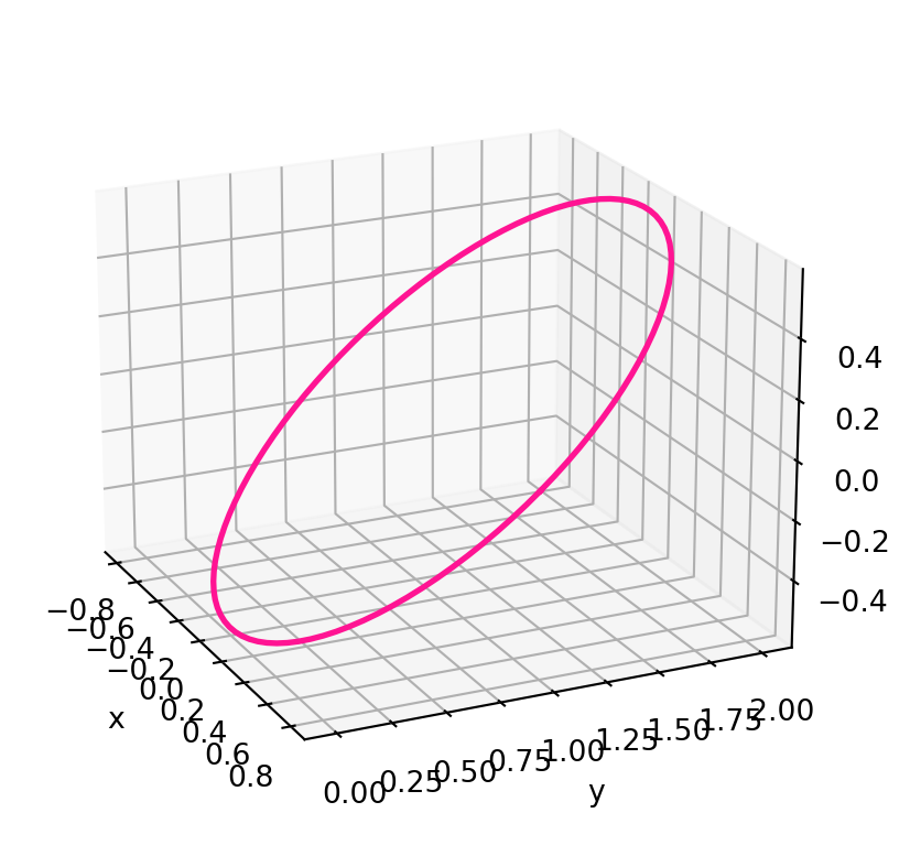
Example 43

Define the space curve $$\gamma \gamma (t):=(\frac{4}{5}\cos (t),1-\sin (t),-\frac{3}{5}\cos (t)),$$ for $t\in \mathbb{R}$. As seen in the plot below, $\gamma \gamma$ is just a Circle which has been rotated an translated. Therefore $\gamma \gamma$ is contained in a plane, and we expect curvature and torsion to be $$\kappa =\frac{1}{R},\tau =0,$$ for some $R>0$, radius of the Circle $\gamma \gamma$. Let us proceed with the calculations: $$\dot{\gamma \gamma }=(-\frac{4}{5}\sin (t),-\cos (t),\frac{3}{5}\sin (t))$$ so that $${\Vert \dot{\gamma \gamma }\Vert }^2=\frac{16}{25}{\sin }^2(t)+{\cos }^2(t)+\frac{9}{25}{\sin }^2(t)=1,$$ showing that $\gamma \gamma$ is regular and unit speed. Further $$\ddot{\gamma \gamma }=(-\frac{4}{5}\cos (t),\sin (t),\frac{3}{5}\cos (t)).$$ As $\gamma \gamma$ is unit speed, we have $$\kappa =\Vert \ddot{\gamma \gamma }\Vert =\frac{16}{25}{\cos }^2(t)+{\sin }^2(t)+\frac{9}{25}{\cos }^2(t)=1.$$ As $\gamma \gamma$ is unit speed, the normal vector is $$\mathbf{n}=\frac{1}{\kappa }\ddot{\gamma \gamma }=(-\frac{4}{5}\cos (t),\sin (t),\frac{3}{5}\cos (t)).$$ We can then compute the binormal $$\begin{array}{rl}\mathbf{b}& =\dot{\gamma \gamma }\times \mathbf{n}\\ & =\left|\begin{array}{ccc}\mathbf{i}& \mathbf{j}& \mathbf{k}\\ -\frac{4}{5}\sin (t)& -\cos (t)& \frac{3}{5}\sin (t)\\ -\frac{4}{5}\cos (t)& \sin (t)& \frac{3}{5}\cos (t)\end{array}\right|\\ & =(-\frac{3}{5}{\cos }^2(t)-\frac{3}{5}{\sin }^2(t),-\frac{12}{25}\cos (t)\sin (t)+\frac{12}{25}\cos (t)\sin (t),-\frac{4}{5}{\sin }^2(t)-\frac{4}{5}{\cos }^2(t))\\ & =(-\frac{3}{5},0,-\frac{4}{5}).\end{array}$$ Therefore $$\dot{\mathbf{b}}=0,$$ and we obtain that the torsion is $$\tau =-\dot{\mathbf{b}}\cdot \mathbf{n}=0.$$

Plot of the curve in example above

2.6 Frenet frame

For a unit speed curve $\gamma \gamma :(a,b)\to {\mathbb{R}}^3$ with non-vanishing curvature we computed the triple $$\{\dot{\gamma \gamma },\mathbf{n},\mathbf{b}\}.$$ We saw that the above is a positive orthonormal basis of ${\mathbb{R}}^3$. We also used this triple to compute curvature $\kappa$ and torsion $\tau$ of $\gamma \gamma$: $$\kappa =\Vert \ddot{\gamma \gamma }\Vert ,\tau =-\dot{\mathbf{b}}\cdot \mathbf{n}.$$ This triple is so important that it has a name.

Definition 44: Frenet frame

Let $\gamma \gamma :(a,b)\to {\mathbb{R}}^3$ be unit speed with $\kappa \ne 0$. The positive orthonormal basis $$\{\dot{\gamma \gamma },\mathbf{n},\mathbf{b}\}$$ is called Frenet frame of $\gamma \gamma$.

We can also define the Frenet frame for regular curves with non-vanishing curvature.

Definition 45

Let $\gamma \gamma :(a,b)\to {\mathbb{R}}^3$ be regular with $\kappa \ne 0$. The Frenet frame of $\gamma \gamma$ is defined as the Frenet frame of a unit speed reparametrization $\widetilde{\gamma \gamma }$ of $\gamma \gamma$.

Remark 46

We should check that the above definition is well-posed:

• Note that $\widetilde{\gamma \gamma }$ is unit speed. Moreover the curvature of ${\kappa }^{\widetilde{\gamma \gamma }}$ is given by $${\kappa }^{\widetilde{\gamma \gamma }}(t)={\kappa }^{\gamma \gamma }(\varphi (t))$$ for some $\varphi$ diffeomorphism. Therefore ${\kappa }^{\widetilde{\gamma \gamma }}\ne 0$ as we are assuming ${\kappa }^{\gamma \gamma }\ne 0$. Therefore the Frenet-Frame of $\widetilde{\gamma \gamma }$ is well defined.

• If $\widehat{\gamma \gamma }$ is another unit speed reparametrization of $\gamma \gamma$, then the Frenet frame generated by $\widehat{\gamma \gamma }$ coincides with the one generated by $\widetilde{\gamma \gamma }$. The proof is left as an exercise.

From the Frenet frame we can define the Frenet-Serret equations.

Theorem 47: Frenet-Serret equations

Let $\gamma \gamma :(a,b)\to {\mathbb{R}}^3$ be unit speed with $\kappa \ne 0$. The Frenet-Serret equations are $$\begin{array}{rl}\ddot{\gamma \gamma }& =\kappa \mathbf{n}\\ \dot{\mathbf{n}}& =-\kappa \dot{\gamma \gamma }+\tau \mathbf{b}\\ \dot{\mathbf{b}}& =-\tau \mathbf{n}\end{array}$$

Proof

The first Frenet-Serret equation $$\begin{array}{}\text{(2.15)}& \ddot{\gamma \gamma }=\kappa \mathbf{n}\end{array}$$ holds by definition of $\mathbf{n}$ and $\kappa$. The third Frenet-Serret equation $$\begin{array}{}\text{(2.16)}& \dot{\mathbf{b}}=-\tau \mathbf{n}\end{array}$$ holds by Proposition 36. Now, recall that in Proposition 35 we have proven $$\begin{array}{}\text{(2.17)}& \mathbf{b}=\dot{\gamma \gamma }\times \mathbf{n},\mathbf{n}=\mathbf{b}\times \dot{\gamma \gamma },\dot{\gamma \gamma }=\mathbf{n}\times \mathbf{b}.\end{array}$$ Differentiating the second equation in (2.17) and using (2.15)-(2.16) we get $$\begin{array}{rlr}\dot{\mathbf{n}}& =\dot{\mathbf{b}}\times \dot{\gamma \gamma }+\mathbf{b}\times \ddot{\gamma \gamma }& \\ & =(-\tau \mathbf{n}\times \dot{\gamma \gamma })+\mathbf{b}\times \kappa \mathbf{n}\\ & =\tau (\dot{\gamma \gamma }\times \mathbf{n})-\kappa (\mathbf{n}\times \mathbf{b})\\ & =\tau \mathbf{b}-\kappa \dot{\gamma \gamma },\end{array}$$ where in the last equality we used the first and third equations in (2.17). The above is exactly the second Frenet-Serret equation.

Remark 48

We can write the Frenet-Serret ODE sysyem in vectorial form. To this end, introduce the matrix $$F:=\left(\begin{array}{ccc}0& \kappa & 0\\ -\kappa & 0& \tau \\ 0& \tau & 0\end{array}\right).$$ It is immediate to check that the Frenet-Serret equations are equivalent to $$\left(\begin{array}{c}\ddot{\gamma \gamma }\\ \dot{\mathbf{n}}\\ \dot{\mathbf{b}}\end{array}\right)=F\left(\begin{array}{c}\dot{\gamma \gamma }\\ \mathbf{n}\\ \mathbf{b}\end{array}\right).$$

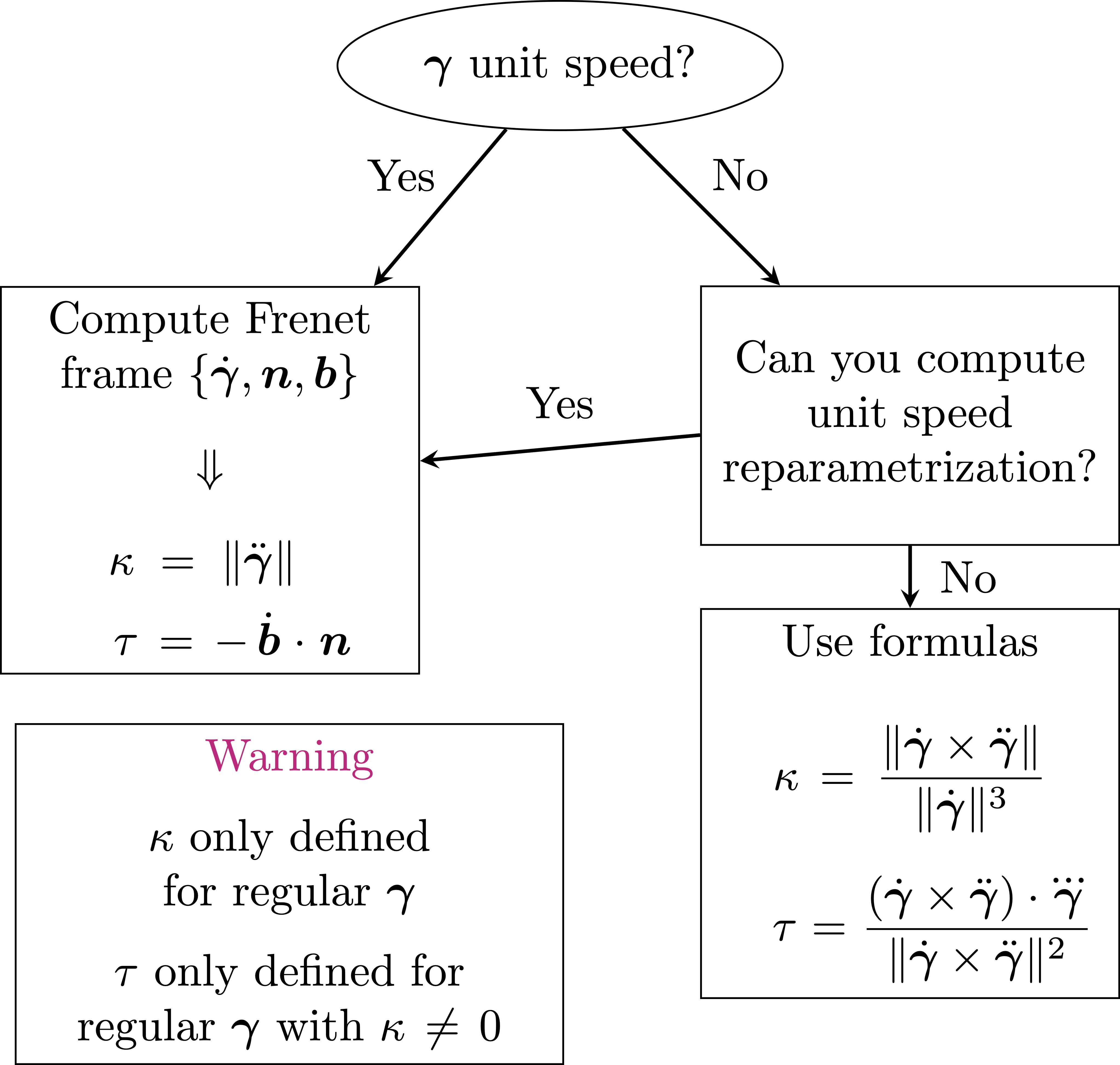
Important: Summary

Recall that:

1. Curvature $\kappa$ is defined only for regular curves.
2. Torsion $\tau$ is defined only for regular curves with non-vanishing $\kappa$.

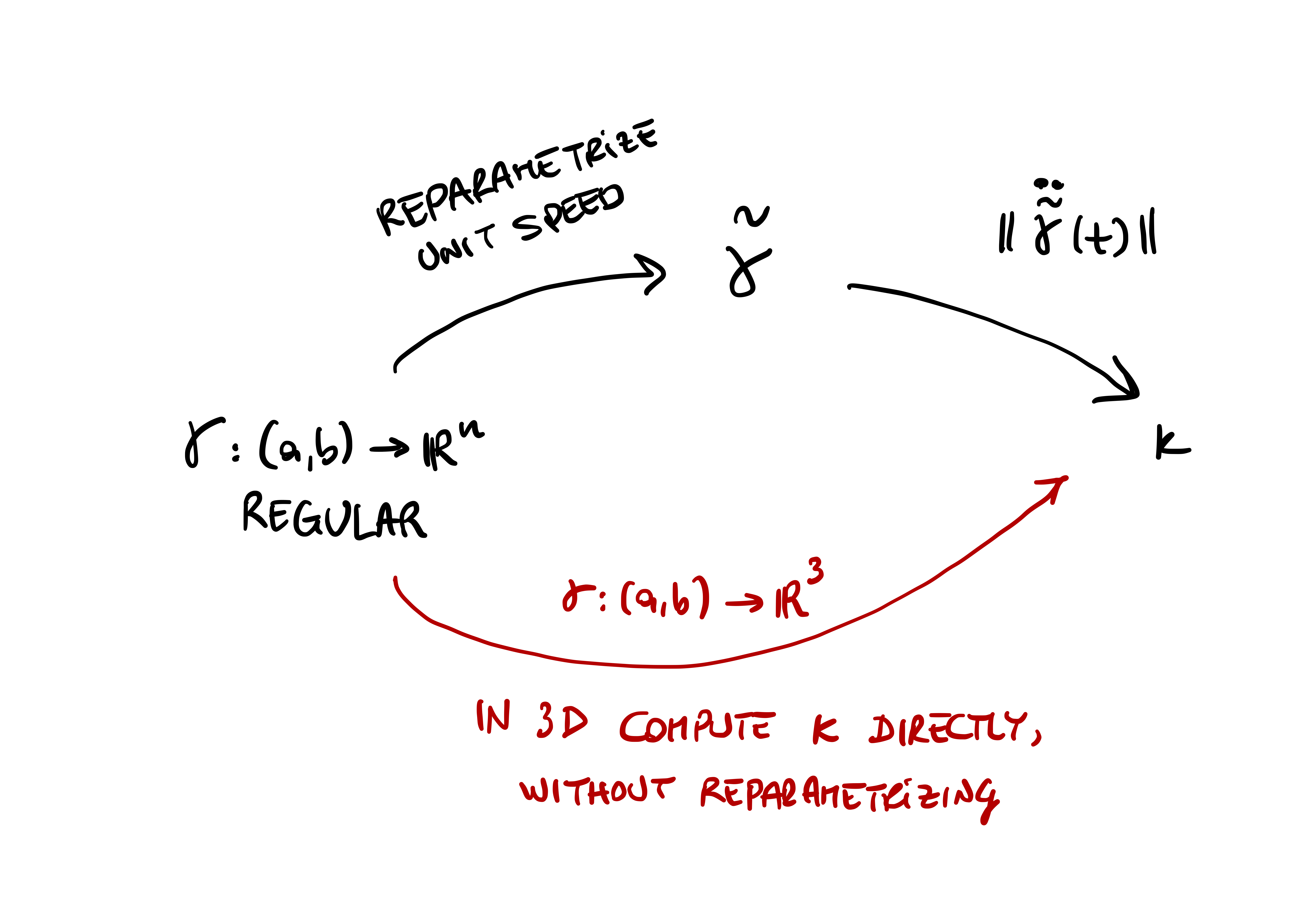
The two strategies for computing $\kappa$ and $\tau$ are discussed in the diagram in Figure 2.4 below.

Figure 2.4: Summary for computing $\kappa$ and $\tau$ for regular curve $\gamma \gamma$.

Let us conclude the section with an example. We compute the Frenet frame of the helix. As a consequence we obtain curvature and torsion.

Example 49: Frenet frame of helix

Consider the helix of radius $1$ and rise $1$ given by $$\gamma \gamma (t)=(\cos (t),\sin (t),t),$$ for $t\in \mathbb{R}$. We now proceed following the diagram at Figure 2.4. We ask the first question: $$\text{Is }\gamma \gamma \text{ unit speed?}$$ We have that $$\dot{\gamma \gamma }(t)=(-\sin (t),\cos (t),1),$$ and therefore $$\Vert \dot{\gamma \gamma }\Vert =\sqrt{2}.$$ This shows that $\gamma \gamma$ is regular but not unit speed. We ask the second question in the diagram: $$\text{Can we find a unit speed reparametrization of }\gamma \gamma \text{?}$$ Let us try. We compute the arc length of $\gamma \gamma$ starting at $t_0=0$ $$s(t):={\int }_0^t\Vert \dot{\gamma \gamma }(u)\Vert du=\sqrt{2}t.$$ The arc length is invertible with $$\psi (t):=s^{-1}(t)=\frac{t}{\sqrt{2}}.$$ Therefore a unit speed reparametrization of $\gamma \gamma$ is given by $$\widetilde{\gamma \gamma }(t):=\gamma \gamma (\psi (t))=(\cos \left(\frac{t}{\sqrt{2}}\right),\sin \left(\frac{t}{\sqrt{2}}\right),\frac{t}{\sqrt{2}}).$$ The next step in the diagram is $$\text{Compute Frenet frame }\{\dot{\gamma \gamma },\mathbf{n},\mathbf{b}\}\text{ and curvature }\kappa \text{, torsion }\tau$$ We compute $$\begin{array}{rl}\dot{\widetilde{\gamma \gamma }}(t)& =\frac{1}{\sqrt{2}}(-\sin \left(\frac{t}{\sqrt{2}}\right),\cos \left(\frac{t}{\sqrt{2}}\right),1)\\ \ddot{\widetilde{\gamma \gamma }}(t)& =\frac{1}{2}(-\cos \left(\frac{t}{\sqrt{2}}\right),-\sin \left(\frac{t}{\sqrt{2}}\right),0)\end{array}$$ Therefore the curvature is $$\kappa (t)=\Vert \ddot{\widetilde{\gamma \gamma }}(t)\Vert =\frac{1}{2}.$$ From the curvature we obtain the principal normal vector $$\mathbf{n}(t)=\frac{1}{\kappa (t)}\ddot{\widetilde{\gamma \gamma }}(t)=(-\cos \left(\frac{t}{\sqrt{2}}\right),-\sin \left(\frac{t}{\sqrt{2}}\right),0).$$ We can now compute the binormal $$\begin{array}{rl}\mathbf{b}(t)& =\dot{\widetilde{\gamma \gamma }}\times \mathbf{n}\\ & =\frac{1}{\sqrt{2}}\left|\begin{array}{ccc}\mathbf{i}& \mathbf{j}& \mathbf{k}\\ -\sin \left(\frac{t}{\sqrt{2}}\right)& \cos \left(\frac{t}{\sqrt{2}}\right)& 1\\ -\cos \left(\frac{t}{\sqrt{2}}\right)& -\sin \left(\frac{t}{\sqrt{2}}\right)& 0\end{array}\right|\\ & =\frac{1}{\sqrt{2}}(\sin \left(\frac{t}{\sqrt{2}}\right),-\cos \left(\frac{t}{\sqrt{2}}\right),1).\end{array}$$ We have therefore computed the Frenet frame of $\gamma \gamma$. 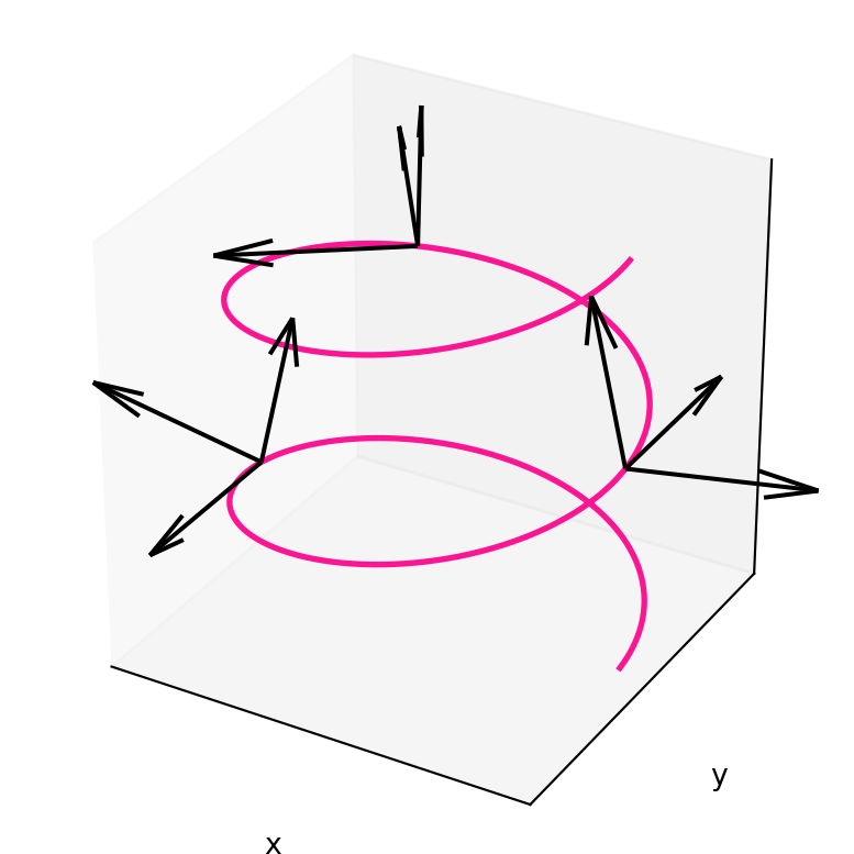This is given by $$\begin{array}{rl}\dot{\widetilde{\gamma \gamma }}(t)& =\frac{1}{\sqrt{2}}(-\sin \left(\frac{t}{\sqrt{2}}\right),\cos \left(\frac{t}{\sqrt{2}}\right),1)\\ \mathbf{n}(t)& =(-\cos \left(\frac{t}{\sqrt{2}}\right),-\sin \left(\frac{t}{\sqrt{2}}\right),0)\\ \mathbf{b}(t)& =\frac{1}{\sqrt{2}}(\sin \left(\frac{t}{\sqrt{2}}\right),-\cos \left(\frac{t}{\sqrt{2}}\right),1).\end{array}$$ See below for a picture of the Frenet frame of the helix. Given the Frenet frame, we can compute the torsion via the formula $$\tau (t)=-\dot{\mathbf{b}}\cdot \mathbf{n}.$$ Indeed, we have $$\dot{\mathbf{b}}=\frac{1}{2}(\cos \left(\frac{t}{\sqrt{2}}\right),-\sin \left(\frac{t}{\sqrt{2}}\right),0)$$ and therefore $$\dot{\mathbf{b}}\cdot \mathbf{n}=\frac{1}{2}(-{\cos }^2\left(\frac{t}{\sqrt{2}}\right)-{\sin }^2\left(\frac{t}{\sqrt{2}}\right))=-\frac{1}{2}.$$ The torsion is then $$\tau (t)=-\dot{\mathbf{b}}\cdot \mathbf{n}=\frac{1}{2}.$$ The Frenet-Frame of the unit-speed Helix is plotted in Figure 2.5.

Figure 2.5: Frenet frame of the helix of radius 1 and rise 1.

2.7 Consequences of Frenet-Serret

The most important consequence of the Frenet-Serret equations is that they allow to fully characterize space curves in terms of curvature and torsion. Precisely, the following theorem holds.

Theorem 50: Characterization of space curves

Let $\kappa ,\tau :\mathbb{R}\to \mathbb{R}$ be smooth functions, with $\kappa >0$. Then:

1. There exists aunit speed curve $\gamma \gamma :\mathbb{R}\to {\mathbb{R}}^3$ such that its curvature ${\kappa }^{\gamma \gamma }$ and torsion ${\tau }^{\gamma \gamma }$ satisfy $${\kappa }^{\gamma \gamma }(t)=\kappa (t),{\tau }^{\gamma \gamma }(t)=\tau (t),\mathrm{\forall }t\in \mathbb{R}.$$

2. Suppose that $\widetilde{\gamma \gamma }:\mathbb{R}\to {\mathbb{R}}^3$ is a unit speed curve such that its curvature ${\tilde{\kappa }}^{\widetilde{\gamma \gamma }}$ and torsion ${\tau }^{\widetilde{\gamma \gamma }}$ satisfy $${\kappa }^{\widetilde{\gamma \gamma }}(t)=\kappa (t),{\tau }^{\widetilde{\gamma \gamma }}(t)=\tau (t),\mathrm{\forall }t\in \mathbb{R}.$$ Then $$\widetilde{\gamma \gamma }=\gamma \gamma$$ up to rotations and translations.

The proof of Theorem 50 is omitted, and it can be found in Theorem 2.3.6 in (Pressley 2010).

Theorem 50 is a very strong result. It is saying two things:

1. If we prescribe curvature and torsion, then there exists a unit speed curve which has such curvature and torsion.

2. If two unit speed curves have same curvature and torsion, then they must be the same curve, up to translations and rotations.

In other words, curvature and torsion fully characterize space curves. This result is the 3D counterpart of Theorem 27, which said that signed curvature characterizes 2D curves.

Example 51

In Example 43 we have considered the unit speed curve $$\gamma \gamma (t):=(\frac{4}{5}\cos (t),1-\sin (t),-\frac{3}{5}\cos (t)),$$ for $t\in [0,2\pi ]$. We have computed that $${\kappa }^{\gamma \gamma }=1,{\tau }^{\gamma \gamma }=0.$$ If we plot $\gamma \gamma$, we clearly see that $\gamma \gamma$ is just obtained by translating and rotating a unit circle, see plot below. Theorem 50 enables us to rigorously prove this claim. Indeed, consider the unit speed circle $$\widetilde{\gamma \gamma }(t):=(\cos (t),\sin (t),0),$$ for $t\in [0,2\pi ]$. In Example 42 we have proven that curvature and torsion are
$${\kappa }^{\widetilde{\gamma \gamma }}=1,{\tau }^{\widetilde{\gamma \gamma }}=1.$$ Therefore $${\kappa }^{\gamma \gamma }={\kappa }^{\widetilde{\gamma \gamma }},{\tau }^{\gamma \gamma }={\tau }^{\widetilde{\gamma \gamma }},$$ and by Theorem 50 we conclude that $\gamma \gamma$ is equal to $\widetilde{\gamma \gamma }$ up to rotations and translations.

Plot of the curve in example above

Another consequence of the Frenet-Serret equations is that they allow us to finally prove the curvature and torsion formulas given in Proposition 19 and Proposition 40. For reader’s convenience we recall these two results.

Proposition 52: Curvature and torsion formulas

Let $\gamma \gamma :(a,b)\to {\mathbb{R}}^3$ be a regular curve. The curvature $\kappa (t)$ of $\gamma \gamma$ at $\gamma \gamma (t)$ is given by $$\kappa (t)=\frac{\Vert \dot{\gamma \gamma }\times \ddot{\gamma \gamma }\Vert }{{\Vert \dot{\gamma \gamma }\Vert }^3}.$$ Suppose in addition that $\gamma \gamma$ has non-vanishing curvature. The torsion $\tau (t)$ of $\gamma \gamma$ at $\gamma \gamma (t)$ is given by $$\tau (t)=\frac{(\dot{\gamma \gamma }\times \ddot{\gamma \gamma })\cdot \stackrel{⃛}{\gamma \gamma }}{{\Vert \dot{\gamma \gamma }\times \ddot{\gamma \gamma }\Vert }^2}.$$

Before proceeding with the proof, we need to establish some notation.

Notation: Compact notation for arc length reparametrization

Suppose $\gamma \gamma :(a,b)\to {\mathbb{R}}^n$ is regular and denote by $$s:(a,b)\to (\tilde{a},\tilde{b}),t\mapsto s(t)$$ its arc length. We already know that in this case $s$ invertible, with inverse $s^{-1}$ giving a unit speed reparametrization $\widetilde{\gamma \gamma }:(\tilde{a},\tilde{b})\to {\mathbb{R}}^n$ of $\gamma \gamma$, defined by $$\widetilde{\gamma \gamma }=\gamma \gamma \circ \psi ,\psi :=s^{-1}:(\tilde{a},\tilde{b})\to (a,b)$$ Sometimes it is more convenient to adopt more compact notation. In the new notation the unit speed reparametrization $\widetilde{\gamma \gamma }$ is denoted by $\gamma \gamma (s)$: $$t\mapsto \widetilde{\gamma \gamma }(t)⇝s\mapsto \gamma \gamma (s).$$ Thus, the reparametrization is denoted with the same symbol $\gamma \gamma$, but this time $\gamma \gamma$ is considered as a function of the arc length parameter $$s\in (\tilde{a},\tilde{b}).$$ We will denote:

• The derivative of $s$ by $$\frac{ds}{dt}$$

• The derivative of $\psi =s^{-1}$ by $$\frac{dt}{ds}.$$

Moreover:

• The derivative of $\gamma \gamma (t)$ is denoted by $$\frac{d\gamma \gamma }{dt}(t)=\dot{\gamma \gamma }(t),t\in (a,b)$$

• The derivative of $\gamma \gamma (s)$ is denoted by $$\frac{d\gamma \gamma }{ds}(s)=\dot{\gamma \gamma }(s),s\in (\tilde{a},\tilde{b}).$$

We also have new notations for the chain rule:

• The chain rule for $\gamma \gamma$ is the old notations is: $$\gamma \gamma (t)=\widetilde{\gamma \gamma }(s(t))⟹\dot{\gamma \gamma }(t)=\dot{\widetilde{\gamma \gamma }}(s(t))\dot{s}(t),t\in (a,b).$$ In the new notations the above chain rule is written $$\frac{d\gamma \gamma }{dt}(t)=\frac{d\gamma \gamma }{ds}(s(t))\frac{ds}{dt}(t),t\in (a,b).$$ We will often omit the dependence on the point $t$ by writing $$\frac{d\gamma \gamma }{ds}=\frac{d\gamma \gamma }{dt}\frac{dt}{ds}.$$

• The chain rule for the reparametrization $\widetilde{\gamma \gamma }$ in the old notation is: $$\widetilde{\gamma \gamma }(t)=\gamma \gamma (\psi (t))⟹\dot{\widetilde{\gamma \gamma }}(t)=\dot{\gamma \gamma }(\psi (t))\dot{\psi }(t),t\in (\tilde{a},\tilde{b}).$$ In the new notations the above chain rule is written $$\frac{d\gamma \gamma }{ds}(s)=\frac{d\gamma \gamma }{dt}(\psi (s))\frac{dt}{ds}(s),s\in (\tilde{a},\tilde{b}),$$ since $\dot{\psi }$ is written $dt/ds$ in the new notations. Without dependence on the point $s$, the above reads $$\frac{d\gamma \gamma }{ds}=\frac{d\gamma \gamma }{dt}\frac{dt}{ds}.$$

Example 53: How to use the new notations

Let $\gamma \gamma$ and $\widetilde{\gamma \gamma }$ be as above. We know that $\widetilde{\gamma \gamma }$ is unit speed. Thus $\gamma \gamma (s)$ is unit speed with respect to $s$, that is, $$\begin{array}{}\text{(2.18)}& \Vert \dot{\gamma \gamma }(s)\Vert =1,\mathrm{\forall }s\in (\tilde{a},\tilde{b}).\end{array}$$ As an exercise, let us check that (2.18) holds, using the new notations. By chain rule we have $$\begin{array}{rl}\Vert \dot{\gamma \gamma }(s)\Vert & =\Vert \frac{d\gamma \gamma }{ds}(s)\Vert \\ & =\Vert \frac{d\gamma \gamma }{dt}(\psi (s))\Vert |\frac{dt}{ds}(s)|\\ & =\Vert \dot{\gamma \gamma }(\psi (s))\Vert |\frac{dt}{ds}(s)|.\end{array}$$ Now, recall that $$\begin{array}{}\text{(2.19)}& \frac{ds}{dt}(t)=\dot{s}(t)=\Vert \dot{\gamma \gamma }(t)\Vert ,\mathrm{\forall }t\in (a,b).\end{array}$$ According to the new notations and the inverse function theorem, $$\frac{dt}{ds}(s)=\frac{1}{({\displaystyle \frac{ds}{dt}}(\psi (s)))}=\frac{1}{\Vert \dot{\gamma \gamma }(\psi (s))\Vert },\mathrm{\forall }s\in (\tilde{a},\tilde{b}),$$ where we used (2.19) evaluated at $t=\psi (s)$. Thus $$\begin{array}{rl}\Vert \dot{\gamma \gamma }(s)\Vert & =\Vert \dot{\gamma \gamma }(\psi (s))\Vert |\frac{dt}{ds}(s)|\\ & =\Vert \dot{\gamma \gamma }(\psi (s))\Vert \frac{1}{\Vert \dot{\gamma \gamma }(\psi (s))\Vert }\\ & =1,\end{array}$$ concluding (2.18).

Let us highlight the main feature of the above notation.

Important: New Notation!

Let $\gamma \gamma :(a,b)\to {\mathbb{R}}^n$ be a regular curve:

1. We denote by $$t\mapsto \gamma \gamma (t),t\in (a,b)$$ the given curve $\gamma \gamma$.

2. We denote by $$s\mapsto \gamma \gamma (s),s\in (\tilde{a},\tilde{b})$$ the arc length reparametrization of the curve $\gamma \gamma$. The parameter $s$ is the arc length parameter. In particular $\gamma \gamma (s)$ is unit speed with respect to $s$.

We will heavily rely on the new notations for proving Proposition 52.

Proof: Proof of Proposition 52

We only prove the formula for $\kappa$, as the one for $\tau$ can be obtained similarly, just with more calculations. For a proof see Proposition 2.3.1 in (Pressley 2010).

Since $\gamma \gamma$ is regular, we can reparametrize $\gamma \gamma$ by arc length $s(t)$. We denote the arc lenght reparametrization by $\gamma \gamma (s)$. We know that $\gamma \gamma (s)$ is unit speed, that is, $$\Vert \frac{d\gamma \gamma }{ds}\Vert =1.$$ Therefore is well define the Frenet frame $$\{\mathbf{t}(s),\mathbf{n}(s),\mathbf{b}(s)\},\mathbf{t}(s):=\dot{\gamma \gamma }(s)=\frac{d\gamma \gamma }{ds}(s).$$ The Frenet-Serret equations are $$\begin{array}{rl}\dot{\mathbf{t}}(s)& =\kappa (s)\mathbf{n}(s)\\ \dot{\mathbf{n}}(s)& =-\kappa (s)\mathbf{t}(s)+\tau (s)\mathbf{b}(s)\\ \dot{\mathbf{b}}(s)& =-\tau (s)\mathbf{n}(s)\end{array}$$ By chain rule $$\frac{d\gamma \gamma }{dt}=\frac{d\gamma \gamma }{ds}\frac{ds}{dt}=\left(\frac{ds}{dt}\right)\mathbf{t}.$$ Differentiating the above we infer $$\begin{array}{rl}\frac{d^2\gamma \gamma }{d{t}^2}& =\frac{d}{dt}\left[\left(\frac{ds}{dt}\right)\mathbf{t}\right]\\ & =\frac{d^{2}s}{d{t}^2}\mathbf{t}+\left(\frac{ds}{dt}\right)\frac{d\mathbf{t}}{dt}.\end{array}$$ By chain rule we have $$\frac{d\mathbf{t}}{dt}=\frac{d\mathbf{t}}{ds}\frac{dt}{ds},$$ and therefore $$\begin{array}{rl}\frac{d^2\gamma \gamma }{d{t}^2}& =\frac{d^{2}s}{d{t}^2}\mathbf{t}+\left(\frac{ds}{dt}\right)\frac{d\mathbf{t}}{dt}\\ & =\frac{d^{2}s}{d{t}^2}\mathbf{t}+{\left(\frac{ds}{dt}\right)}^2\frac{d\mathbf{t}}{ds}.\end{array}$$ Hence $$\begin{array}{rl}\dot{\gamma \gamma }(t)\times \ddot{\gamma \gamma }(t)& =\frac{d\gamma \gamma }{dt}\times \frac{d^2\gamma \gamma }{d{t}^2}\\ & =\left(\frac{ds}{dt}\right)\mathbf{t}\times [\frac{d^{2}s}{d{t}^2}\mathbf{t}+{\left(\frac{ds}{dt}\right)}^2\frac{d\mathbf{t}}{ds}]\\ & =[\left(\frac{ds}{dt}\right)\left(\frac{d^{2}s}{d{t}^2}\right)\mathbf{t}\times \mathbf{t}]+[{\left(\frac{ds}{dt}\right)}^3\mathbf{t}\times \frac{d\mathbf{t}}{ds}]\\ & ={\left(\frac{ds}{dt}\right)}^3\mathbf{t}\times \frac{d\mathbf{t}}{ds},\end{array}$$ since $\mathbf{t}\times \mathbf{t}=0$ by the properties of the cross product. Now we recall that $$\frac{d\mathbf{t}}{ds}=\kappa (s)\mathbf{n}(s)$$ by the first Frenet-Serret equation. Moreover $$\frac{ds}{dt}(t)={\Vert \dot{\gamma \gamma }(t)\Vert }^2.$$ Therefore $$\begin{array}{rl}\dot{\gamma \gamma }(t)\times \ddot{\gamma \gamma }(t)& ={\left(\frac{ds}{dt}\right)}^3\mathbf{t}\times \frac{d\mathbf{t}}{ds}\\ & ={\Vert \dot{\gamma \gamma }(t)\Vert }^3\kappa (s(t))\mathbf{t}\times \mathbf{n}\\ & ={\Vert \dot{\gamma \gamma }(t)\Vert }^3\kappa (s(t))\mathbf{b},\end{array}$$ where in the last line we used the definition of $\mathbf{b}$ $$\mathbf{b}(s)=\dot{\gamma \gamma }(s)\times \mathbf{n}(s)=\mathbf{t}(s)\times \mathbf{n}(s).$$ We can now take the norms and obtain $$\begin{array}{rl}\Vert \dot{\gamma \gamma }(t)\times \ddot{\gamma \gamma }(t)\Vert & ={\Vert \dot{\gamma \gamma }(t)\Vert }^3\kappa (s(t))\Vert \mathbf{b}\Vert \\ & ={\Vert \dot{\gamma \gamma }(t)\Vert }^3\kappa (s(t))\end{array}$$ using that $\Vert \mathbf{b}\Vert =1$. As $\gamma \gamma$ is regular, we can divide by ${\Vert \dot{\gamma \gamma }(t)\Vert }^3$ and obtain $$\kappa (s(t))=\frac{\Vert \dot{\gamma \gamma }(t)\times \ddot{\gamma \gamma }(t)\Vert }{{\Vert \dot{\gamma \gamma }(t)\Vert }^3}.$$ Recalling that the curvature of $\gamma \gamma$ at $t$ is defined as the curvature of $\gamma \gamma (s)$ at $s(t)$, we conclude that the above is the desired formula.

We now state and prove two more results which directly follow from the Frenet-Serret equations. They state, respectivley:

1. A curve has torsion $\tau =0$ if and only if it is contained in a plane.

2. A curve has constant curvature and zero torsion if and only if it is part of a circle.

Before proceeding, we recall the following.

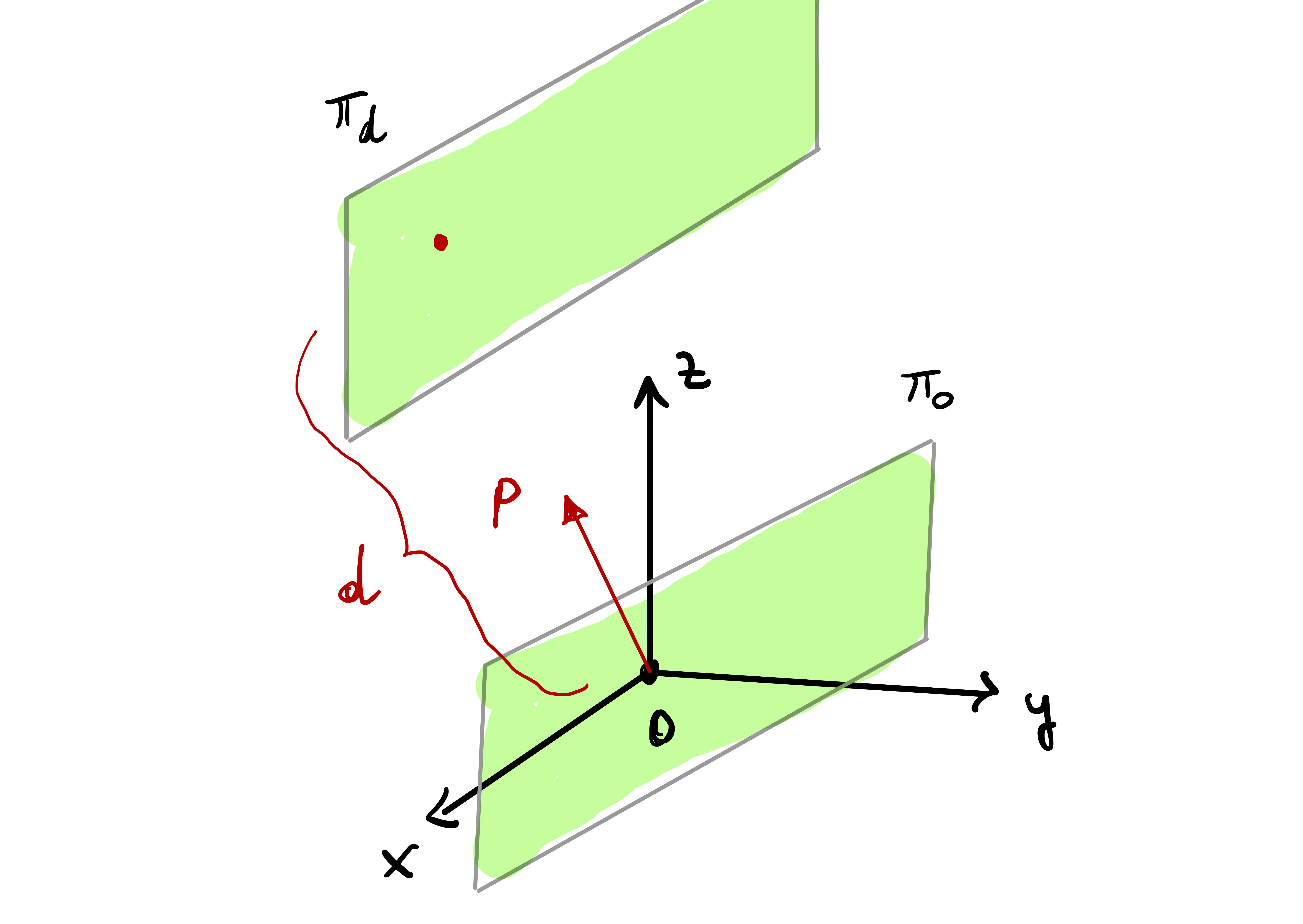
Remark 54: Equation of a plane

The general equation of a plane $\pi {\pi }_d$ in ${\mathbb{R}}^3$ is given by

$$\pi {\pi }_d=\{\mathbf{x}\in {\mathbb{R}}^3:\mathbf{x}\cdot \mathbf{P}=d\},$$ for some vector $\mathbf{P}\in {\mathbb{R}}^3$ and scalar $d\in \mathbb{R}$. Note that:

• If $d=0$, the condition $$\mathbf{x}\cdot \mathbf{P}=0$$ is saying that the plane $\pi {\pi }_0$ contains all the points $\mathbf{x}$ in ${\mathbb{R}}^3$ which are orthogonal to $\mathbf{P}$. In particular $\pi {\pi }_0$ contains the origin $00$.

• If $d\ne 0$, then $\pi {\pi }_d$ is the translation of $\pi {\pi }_0$ by the quantity $d$ in direction $\mathbf{P}$.

In both cases, $\mathbf{P}$ is the normal vector to the plane, as shown in Figure 2.6 below.

Figure 2.6: The plane $\pi {\pi }_0$ is the set of points of ${\mathbb{R}}^3$ orthogonal to $\mathbf{P}$. The plane $\pi {\pi }_d$ is obtained by translating $\pi {\pi }_0$ by a quantity $d$ in direction $\mathbf{P}$.

Proposition 55

Let $\gamma \gamma :(a,b)\to {\mathbb{R}}^3$ be regular and such that $\kappa \ne 0$. They are equivalent:

1. The torsion of $\gamma \gamma$ satisfies $\tau (t)=0$ for all $t\in (a,b)$.

2. The image of $\gamma \gamma$ is contained in a plane, that is, there exists a vector $\mathbf{P}\in {\mathbb{R}}^3$ and a scalar $d\in \mathbb{R}$ such that $$\gamma \gamma (t)\cdot \mathbf{P}=d,\mathrm{\forall }t\in (a,b).$$

Proof

Without loss of generality we can assume that $\gamma \gamma$ is unit speed. Indeed, if we were to consider $\widetilde{\gamma \gamma }$ a unit speed reparametrization of $\gamma \gamma$, then

• $\widetilde{\gamma \gamma }$ would still be contained in the same plane in which $\gamma \gamma$ is contained.
• The torsion of $\widetilde{\gamma \gamma }$ would not change, i.e., it would still be identically zero.

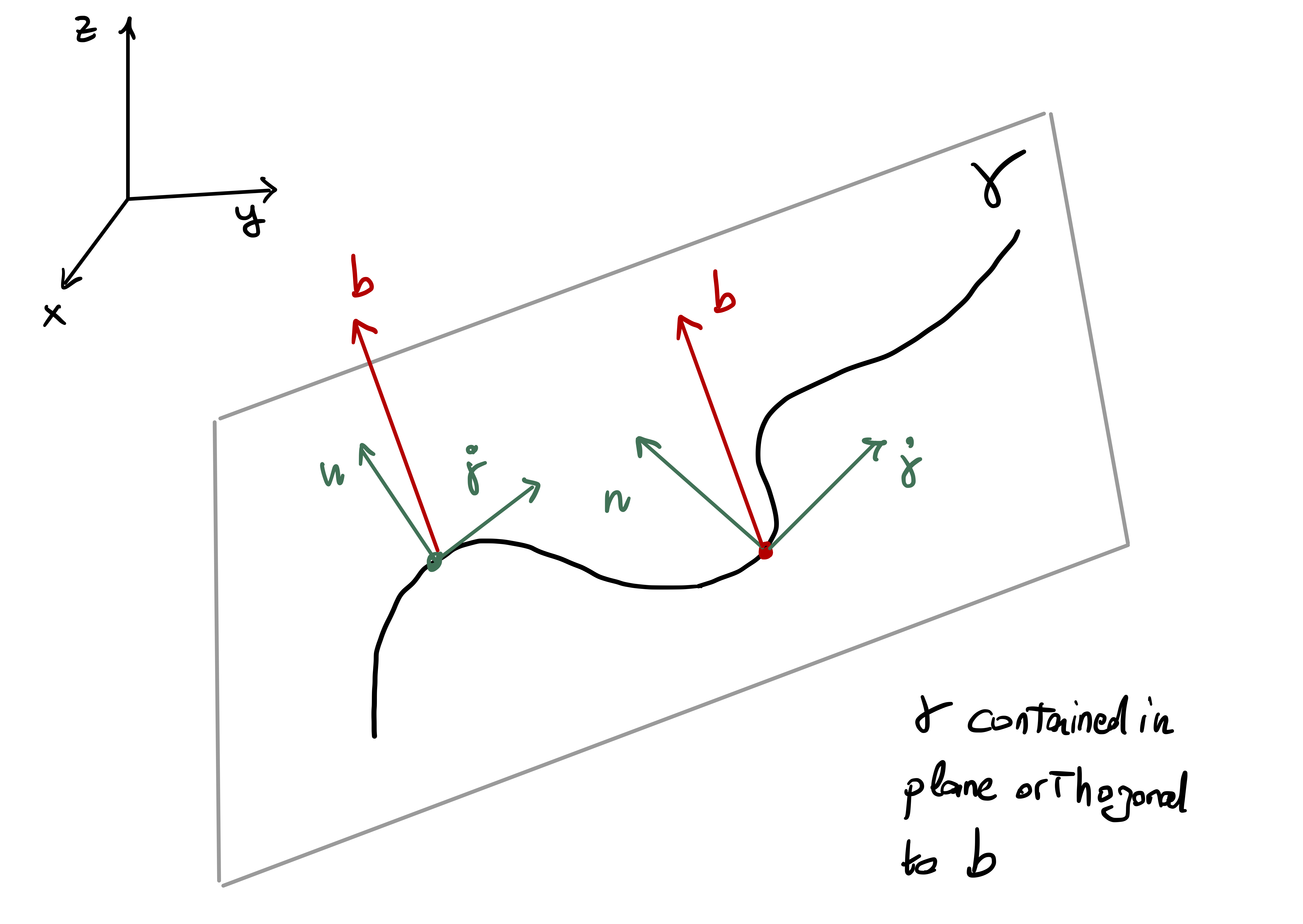
Thefore the Frenet frame of $\gamma \gamma$ exists. We denote it by $$\{\dot{\gamma \gamma }(t),\mathbf{n}(t),\mathbf{b}(t)\}.$$

Step 1. Suppose that $\tau =0$ for all $t$. By the Frenet-Serret equations we have $$\dot{\mathbf{b}}=-\tau (t)\mathbf{n}=00,$$ so that $\mathbf{b}(t)$ is constant. As by definition $$\mathbf{b}=\dot{\gamma \gamma }\times \mathbf{n},$$ we conclude that the vectors $\dot{\gamma \gamma }(t)$ and $\mathbf{n}(t)$ always span the same plane, which has constant normal vector $\mathbf{b}$. Intuition suggests that $\gamma \gamma$ should be contained in such plane, see Figure Figure 2.7 below. Indeed, recall that the Frenet frame is orthonormal. Hence $$\dot{\gamma \gamma }\cdot \mathbf{b}=0,\mathrm{\forall }t\in (a,b).$$ Then $$\frac{d}{dt}(\gamma \gamma \cdot \mathbf{b})=\dot{\gamma \gamma }\cdot \mathbf{b}+\gamma \gamma \cdot \dot{\mathbf{b}}=0,\mathrm{\forall }t\in (a,b),$$ since $\dot{\mathbf{b}}=0$. Thus $\gamma \gamma \cdot \mathbf{b}$ is a constant scalar function, meaning that there exists costant $d\in \mathbb{R}$ such that $$\gamma \gamma (t)\cdot \mathbf{b}=d,\mathrm{\forall }t\in (a,b).$$ The says that $\gamma \gamma$ is contained in a plane.

Step 2. Suppose that $\gamma \gamma$ is contained in a plane. Hence there exists $\mathbf{P}\in {\mathbb{R}}^3$ and $d\in \mathbb{R}$ such that $$\gamma \gamma (t)\cdot \mathbf{P}=d,\mathrm{\forall }t\in (a,b).$$ We can differentiate the above equation twice to obtain $$\dot{\gamma \gamma }\cdot \mathbf{P}=0,\ddot{\gamma \gamma }\cdot \mathbf{P}=0,$$ where we used that $\mathbf{P}$ and $d$ are constant. By Frenet-Serret we have $$\ddot{\gamma \gamma }(t)=\kappa (t)\mathbf{n}(t).$$ Therefore the already proven relation $\ddot{\gamma \gamma }\cdot \mathbf{P}=0$ implies $$\kappa (t)\mathbf{n}(t)\cdot \mathbf{P}=0.$$ As we are assuming $\kappa \ne 0$, we deduce that $$\mathbf{n}(t)\cdot \mathbf{P}=0,\mathrm{\forall }t\in (a,b).$$ We have shown that $\dot{\gamma \gamma }(t)$ and $\mathbf{n}(t)$ are both orthogonal to $\mathbf{P}$. Since $\mathbf{b}(t)$ is orthogonal to $\dot{\gamma \gamma }(t)$ and $\mathbf{n}(t)$, we conclude that $\mathbf{b}(t)$ is parallel to $\mathbf{P}$. Hence, there exists $\lambda (t)\in \mathbb{R}$ such that $$\begin{array}{}\text{(2.20)}& \mathbf{b}(t)=\lambda (t)\mathbf{P}\mathrm{\forall }t\in (a,b).\end{array}$$ Since $\Vert \mathbf{b}\Vert =1$ and $\mathbf{P}$ is constant, from (2.20) we conclude that $\lambda (t)$ is constant. Differentiating (2.20) we obtain $$\dot{\mathbf{b}}(t)=0,\mathrm{\forall }t\in (a,b).$$ By definition of torsion we thus have $$\tau (t)=-\dot{\mathbf{b}}\cdot \mathbf{n}(t)=0,\mathrm{\forall }t\in (a,b).$$

Figure 2.7: If $\mathbf{b}$ is constant, then $\gamma \gamma$ lies in the plane spanned by $\dot{\gamma \gamma }$ and $\mathbf{n}$.

Proposition 56

Let $\gamma \gamma :(a,b)\to {\mathbb{R}}^3$ be a unit speed curve. They are equivalent:

1. The image of $\gamma \gamma$ is contained in a circle of radius $1/c$.

2. The curvature and torsion of $\gamma \gamma$ satisfy $$\kappa (t)=c,\tau (t)=0,\mathrm{\forall }t\in (a,b),$$ for some constant $c\in \mathbb{R}$.

Proposition 56 is actually a consequence of Theorem 50, and of the fact that we have computed that for a circle of radius $R$ one has $$\kappa =\frac{1}{R},\tau =0.$$ Therefore, by Theorem 50, every unit speed curve $\gamma \gamma$ with constant curvature and torsion must be equal to a circle, up to rigid motions.

Nevertheless, we still give a proof of Proposition 56, to show yet another application of the Frenet-Serret equations.

Proof

Step 1. Suppose the image of $\gamma \gamma$ is contained in a circle of radius $1/c$. Then, up to a translation, $\gamma \gamma$ is parametrized by $$\gamma \gamma (t)=(\frac{1}{c}\cos (t),\frac{1}{c}\sin (t),0)$$ for $t$ in some interval $(\tilde{a},\tilde{b})$. We have already seen that in this case $$\kappa =c,\tau =0,$$ concluding the proof.

Step 2. Suppose that $$\kappa (t)=c,\tau (t)=0,\mathrm{\forall }t\in (a,b),$$ for some constant $c\in \mathbb{R}$. Since $\gamma \gamma$ is unit speed, its Frenet-Serret equations are: $$\begin{array}{rl}\ddot{\gamma \gamma }& =\kappa \mathbf{n}=c\mathbf{n}\\ \dot{\mathbf{n}}& =-\kappa \dot{\gamma \gamma }+\tau \mathbf{b}=-c\dot{\gamma \gamma }\\ \dot{\mathbf{b}}& =-\tau \mathbf{n}=0\end{array}$$ In particular $\dot{\mathbf{b}}=0$ and so $\mathbf{b}$ is a constant vector. As seen in the proof Proposition 55, this implies that $\gamma \gamma$ is contained in a plane $\pi \pi$ orthogonal to $\mathbf{b}$, see Figure 2.7. As $c$ is constant we get $$\frac{d}{dt}(\gamma \gamma +\frac{1}{c}\mathbf{n})=\dot{\gamma \gamma }+\frac{1}{c}\dot{\mathbf{n}}=\dot{\gamma \gamma }-\frac{1}{c}c\dot{\gamma \gamma }=0,$$ where we used the second Frenet-Serret equation. Therefore $$\gamma \gamma (t)+\frac{1}{c}\mathbf{n}(t)=\mathbf{p},t\in (a,b),$$ for some constant point $\mathbf{p}\in {\mathbb{R}}^3$. In particular $$\Vert \gamma \gamma (t)-\mathbf{p}\Vert =\Vert -\frac{1}{c}\mathbf{n}(t)\Vert =\frac{1}{c},$$ since $\mathbf{n}$ is a unit vector. The above shows that $\gamma \gamma$ is contained in a sphere of radius $1/c$ and center $\mathbf{p}$. In formulas: $$\gamma \gamma ((a,b))\subset \mathcal{S}:=\{\mathbf{x}\in {\mathbb{R}}^3:\Vert \mathbf{x}-\mathbf{p}\Vert =1/c\}.$$ The intersection of $\mathcal{S}$ with the plane $\pi \pi$ is a circle $\mathcal{C}$ with some radius $R$. Since $$\gamma \gamma ((a,b))\subset \pi \pi ,\gamma \gamma ((a,b))\subset \mathcal{S},$$ this implies $$\begin{array}{}\text{(2.21)}& \gamma \gamma ((a,b))\subset \pi \pi \cap \mathcal{S}=\mathcal{C}.\end{array}$$ Thus $\gamma \gamma$ parametrizes part of $\mathcal{C}$. From Step 1 it follows that the curvature and torsion of $\gamma \gamma$ must satisfy $$\kappa =\frac{1}{R},\tau =0.$$ Since we already know that $\kappa =c$, we conclude that $R=1/c$. Therefore the circle $\mathcal{C}$ has radius $1/c$ and the thesis follows by (2.21).

do Carmo, Manfredo P. 2017. Differential Geometry of Curves and Surfaces. Second Edition. Dover Books on Mathematics.

Pressley, Andrew. 2010. Elementary Differential Geometry. Second Edition. Springer.