    Pearson's Chi-squared test

data:  counts
X-squared = 228.11, df = 2, p-value < 2.2e-16Statistical Models
Lecture 6
Lecture 6:
Chi-squared test &
Least Squares
Outline of Lecture 6
- Chi-squared test of independence
- Worked Example
- Lists
- Data Frames
- Data Entry
- Least squares
- Worked Example
Part 1:
Chi-squared test
of independence
Testing for independence
| Owned | Rented | Total | |
|---|---|---|---|
| North West | 2180 | 871 | 3051 |
| London | 1820 | 1400 | 3220 |
| South West | 1703 | 614 | 2317 |
| Total | 5703 | 2885 | 8588 |
Consider a two-way contingency table as above
To each person we associate two categories:
- Residential Status: Rental or Owned
- Region in which they live: NW, London, SW
Testing for independence
| Owned | Rented | Total | |
|---|---|---|---|
| North West | 2180 | 871 | 3051 |
| London | 1820 | 1400 | 3220 |
| South West | 1703 | 614 | 2317 |
| Total | 5703 | 2885 | 8588 |
- One possible question is:
- Does Residential Status depend on Region?
- In other words: Are rows and columns dependent?
Testing for independence
| Owned | Rented | Total | |
|---|---|---|---|
| North West | 2180 | 871 | 3051 |
| London | 1820 | 1400 | 3220 |
| South West | 1703 | 614 | 2317 |
| Total | 5703 | 2885 | 8588 |
- Looking at the data, it seems clear that:
- London: Rentals are almost comparable to Owned
- NW and SW: Rentals are almost a third of Owned
- It appears Residential Status and Region are dependent features
- Goal: Formulate test for independence
Testing for independence
| Y = 1 | \ldots | Y = C | Totals | |
|---|---|---|---|---|
| X = 1 | O_{11} | \ldots | O_{1C} | O_{1+} |
| \cdots | \cdots | \cdots | \cdots | \cdots |
| X = R | O_{R1} | \ldots | O_{RC} | O_{R+} |
| Totals | O_{+1} | \ldots | O_{+C} | m |
Consider the general two-way contingency table as above
They are equivalent:
- Rows and columns are independent
- Random variables X and Y are independent
Testing for independence
| Y = 1 | \ldots | Y = C | Totals | |
|---|---|---|---|---|
| X = 1 | O_{11} | \ldots | O_{1C} | O_{1+} |
| \cdots | \cdots | \cdots | \cdots | \cdots |
| X = R | O_{R1} | \ldots | O_{RC} | O_{R+} |
| Totals | O_{+1} | \ldots | O_{+C} | m |
Hence, testing for independece means testing following hypothesis: \begin{align*} & H_0 \colon X \, \text{ and } \, Y \, \text{ are independent } \\ & H_1 \colon X \, \text{ and } \, Y \, \text{ are not independent } \end{align*}
We need to quantify H_0 and H_1
Testing for independence
| Y = 1 | \ldots | Y = C | Totals | |
|---|---|---|---|---|
| X = 1 | p_{11} | \ldots | p_{1C} | p_{1+} |
| \cdots | \cdots | \cdots | \cdots | \cdots |
| X = R | p_{R1} | \ldots | p_{RC} | p_{R+} |
| Totals | p_{+1} | \ldots | p_{+C} | 1 |
R.v. X and Y are independent iff cell probabilities factor into marginals p_{ij} = P(X = i , Y = j) = P(X = i) P (Y = j) = p_{i+}p_{+j}
Therefore the hypothesis test for independence becomes \begin{align*} & H_0 \colon p_{ij} = p_{i+}p_{+j} \quad \text{ for all } \, i = 1, \ldots , R \, \text{ and } \, j = 1 ,\ldots C \\ & H_1 \colon p_{ij} \neq p_{i+}p_{+j} \quad \text{ for some } \, (i,j) \end{align*}
Expected counts
Assume the null hypothesis is true H_0 \colon p_{ij} = p_{i+}p_{+j} \quad \text{ for all } \, i = 1, \ldots , R \, \text{ and } \, j = 1 ,\ldots C
Under H_0, the expected counts become E_{ij} = m p_{ij} = p_{i+}p_{+j}
We need a way to estimate the marginal probabilities p_{i+} and p_{+j}
Estimating marginal probabilities
Goal: Estimate marginal probabilities p_{i+} and p_{+j}
By definition we have p_{i+} = P( X = i )
Hence p_{i+} is probability of and observation to be classified in i-th row
Estimate p_{i+} with the proportion of observations classified in i-th row p_{i+} := \frac{o_{i+}}{m} = \frac{ \text{Number of observations in } \, i\text{-th row} }{ \text{ Total number of observations} }
Estimating marginal probabilities
Goal: Estimate marginal probabilities p_{i+} and p_{+j}
Similarly, by definition p_{+j} = P( Y = j )
Hence p_{+j} is probability of and observation to be classified in j-th column
Estimate p_{+j} with the proportion of observations classified in j-th column p_{+j} := \frac{o_{+j}}{m} = \frac{ \text{Number of observations in } \, j\text{-th column} }{ \text{ Total number of observations} }
\chi^2 statistic for testing independence
Summary: The marginal probabilities are estimated with p_{i+} := \frac{o_{i+}}{m} \qquad \qquad p_{+j} := \frac{o_{+j}}{m}
Therefore the expected counts become E_{ij} = m p_{ij} = m p_{i+} p_{+j} = m \left( \frac{o_{i+}}{m} \right) \left( \frac{o_{+j}}{m} \right) = \frac{o_{i+} \, o_{+j}}{m}
By the Theorem in Slide 20, the chi-squared statistics satisfies \chi^2 = \sum_{i=1}^R \sum_{j=1}^C \frac{ (O_{ij} - E_{ij})^2 }{ E_{ij} } \ \approx \ \chi^2_{RC - 1 - {\rm fitted}}
We need to compute the number of fitted parameters
We estimate the first R-1 row marginals by p_{i+} := \frac{o_{i+}}{m} \,, \qquad i = 1 , \ldots, R - 1
Since the marginals p_{i+} sum to 1, we can obtain p_{R+} by p_{R+} = 1 - p_{1+} - \ldots - p_{(R-1)+} = 1 - \frac{o_{1+}}{m} - \ldots - \frac{o_{(R-1)+}}{m}
Similarly, we estimate the first C-1 column marginals by p_{+j} = \frac{o_{+j}}{m} \,, \qquad j = 1, \ldots, C - 1
Since the marginals p_{+j} sum to 1, we can obtain p_{+C} by p_{+C} = 1 - p_{+1} - \ldots - p_{+(C-1)} = 1 - \frac{o_{+1}}{m} - \ldots - \frac{o_{+(C-1)}}{m}
In total, we only have to estimate (R - 1) + (C - 1 ) = R + C - 2 parameters
Therefore, the fitted parameters are {\rm fitted} = R + C - 2
Consequently, the degrees of freedom are \begin{align*} RC - 1 - {\rm fitted} & = RC - 1 - R - C + 2 \\ & = RC - R - C + 1 \\ & = (R - 1)(C - 1) \end{align*}
\chi^2 statistic for testing independence
Conclusion
Assume the null hypothesis of row and column independence H_0 \colon p_{ij} = p_{i+}p_{+j} \quad \text{ for all } \, i = 1, \ldots , R \, \text{ and } \, j = 1 ,\ldots C
Suppose the counts are O \sim \mathop{\mathrm{Mult}}(m,p), and expected counts are E_{ij} = \frac{o_{i+} \, o_{+j}}{m}
By the previous slides, and Theorem in Slide 20 we have that \chi^2 = \sum_{i=1}^R \sum_{j=1}^C \frac{ (O_{ij} - E_{ij})^2 }{ E_{ij} } \approx \ \chi_{RC - 1 - {\rm fitted} }^2 = \chi_{(R-1)(C-1)}^2
\chi^2 statistic for testing independence
Quality of approximation
The chi-squared approximation \chi^2 = \sum_{i=1}^R \sum_{j=1}^C \frac{ (O_{ij} - E_{ij})^2 }{ E_{ij} } \approx \ \chi_{(R-1)(C-1)}^2 is good if E_{ij} \geq 5 \quad \text{ for all } \,\, i = 1 , \ldots , R \, \text{ and } j = 1, \ldots, C
The chi-squared test of independence
Sample:
We draw m individuals from population
Each individual can be of type (i,j), where
- i = 1 , \ldots ,R
- j = 1 , \ldots ,C
- Total of n = RC types
O_{ij} denotes the number of items of type (i,j) drawn
p_{ij} is probability of observing type (i,j)
p = (p_{ij})_{ij} is probability matrix
The matrix of counts O = (o_{ij})_{ij} has multinomial distribution \mathop{\mathrm{Mult}}(m,p)
Data: Matrix of counts, represented by two-way contigency table
| Y = 1 | \ldots | Y = C | Totals | |
|---|---|---|---|---|
| X = 1 | o_{11} | \ldots | o_{1C} | o_{1+} |
| \cdots | \cdots | \cdots | \cdots | \cdots |
| X = R | o_{R1} | \ldots | o_{RC} | o_{R+} |
| Totals | o_{+1} | \ldots | o_{+C} | m |
Hypothesis test: We test for independence of rows and columns \begin{align*} & H_0 \colon X \, \text{ and } \, Y \, \text{ are independent } \\ & H_1 \colon X \, \text{ and } \, Y \, \text{ are not independent } \end{align*}
Procedure: 3 Steps
- Calculation:
Compute marginal and total counts o_{i+} := \sum_{j=1}^C o_{ij} \,, \qquad o_{+j} := \sum_{i=1}^R o_{ij} \,, \qquad m = \sum_{i=1}^R o_{i+} = \sum_{j=1}^C o_{+j}
Compute the expected counts E_{ij} = \frac{o_{i+} \, o_{+j} }{ m }
Compute the chi-squared statistic \chi^2 = \sum_{i=1}^R \sum_{j=1}^C \frac{ (o_{ij} - E_{ij})^2 }{E_{ij}}
- Statistical Tables or R:
- Check that E_{ij} \geq 5 for all i and j
- We fitted R + C - 2 parameters. By the Theorem we get \chi^2 \ \approx \ \chi_{\rm df}^2 \,, \qquad {\rm df} = {\rm degrees \,\, freedom} = (R-1)(C-1)
- Find critical value \chi^2_{\rm df} (0.05) in chi-squared Table 2
- Alternatively, compute p-value in R
- Interpretation: Reject H_0 when either p < 0.05 \qquad \text{ or } \qquad \chi^2 \in \,\,\text{Rejection Region}
| Alternative | Rejection Region | p-value |
|---|---|---|
| X and Y not independent | \chi^2 > \chi^2_{\rm{df}}(0.05) | P(\chi_{\rm df}^2 > \chi^2) |
The chi-squared test of independence in R
- Store each row of counts (o_{i1}, o_{i2}, \ldots, o_{iC}) in R vector
row_i <- c(o_i1, o_i2, ..., o_iC)
- The matrix of counts o = (o_{ij})_{ij} is obtained by assembling rows into a matrix
counts <- rbind(row_1, ..., row_R)
- Perform a chi-squared goodness-of-fit test on
countswithnull.p
| Alternative | R command |
|---|---|
| X and Y are independent | chisq.test(counts) |
- Read output: In particular look for the p-value
Note: Compute Monte Carlo p-value with option simulate.p.value = TRUE
Part 2:
Worked Example
Example: Residential Status and Region
| Owned | Rented | Total | |
|---|---|---|---|
| North West | 2180 | 871 | 3051 |
| London | 1820 | 1400 | 3220 |
| South West | 1703 | 614 | 2317 |
| Total | 5703 | 2885 | 8588 |
People are sampled at random in NW, London and SW
To each person we associate two categories:
- Residential Status: Rental or Owned
- Region in which they live: NW, London, SW
Question: Are Residential Status and Region independent?
Chi-squared test of independence by hand
- Calculation:
- Total and marginal counts are already provided in the table
| Owned | Rented | Tot | |
|---|---|---|---|
| NW | 2180 | 871 | o_{1+} = 3051 |
| Lon | 1820 | 1400 | o_{2+} = 3220 |
| SW | 1703 | 614 | o_{3+} = 2317 |
| Tot | o_{+1} = 5703 | o_{+2} = 2885 | m = 8588 |
- Compute the estimated expected counts E_{ij} = \dfrac{o_{i+} \, o_{+j} }{ m }
| Owned | Rented | Tot | |
|---|---|---|---|
| NW | \frac{3051{\times}5703}{8588} \approx 2026 | \frac{3051{\times}2885}{8588} \approx 1025 | o_{1+} = 3051 |
| Lon | \frac{3220{\times}5703}{8588} \approx 2138 | \frac{3220{\times}2885}{8588} \approx 1082 | o_{2+} = 3220 |
| SW | \frac{2317{\times}5703}{8588} \approx 1539 | \frac{2317{\times}2885}{8588} \approx 778 | o_{3+} = 2317 |
| Tot | o_{+1} = 5703 | o_{+2} = 2885 | m = 8588 |
- Compute the chi-squared statistic \begin{align*} \chi^2 & = \sum_{i=1}^R \sum_{j=1}^C \frac{ (o_{ij} - E_{ij})^2 }{E_{ij}} \\ & = \frac{(2180-2026.066)^2}{2026.066} + \frac{(871-1024.934)^2}{1024.934} \\ & \, + \frac{(1820-2138.293)^2}{2138.293}+\frac{(1400-1081.707)^2}{1081.707} \\ & \, + \frac{(1703-1538.641)^2}{1538.641}+\frac{(614-778.359)^2}{778.359} \\ & = 11.695+23.119 \\ & \, + 47.379+93.658 \\ & \, + 17.557+34.707 \\ & = 228.12 \qquad (2\ \text{d.p.}) \end{align*}
- Statistical Tables:
- Rows are R = 3 and columns are C = 2
- Degrees of freedom are \, {\rm df} = (R - 1)(C - 1) = 2
- We clearly have E_{ij} \geq 5 for all i and j
- Therefore, the following approximation holds \chi^2 \ \approx \ \chi_{(R - 1)(C - 1)}^2 = \chi_{2}^2
- In chi-squared Table 2, we find critical value \chi^2_{2} (0.05) = 5.99
- Interpretation:
- We have that \chi^2 = 228.12 > 5.99 = \chi_{2}^2 (0.05)
- Therefore we rejct H_0, meaning that rows and columns are dependent
- There is evidence (p < 0.05) that Residential Status depends on Region
- By rescaling table values, we can compute the table of percentages
| Owned | Rented | |
|---|---|---|
| North West | 71.5\% | 28.5\% |
| London | 56.5\% | 43.5\% |
| South West | 73.5\% | 26.5\% |
- The above suggests that in London fewer homes are Owned and more Rented
Chi-squared test of independence in R
- Test can be performed using code independence_test.R
Output
- Running the code, we obtain
- This confirms the chi-squared statistic computed by hand \chi^2 = 228.11
- It also confirms the degrees of freedom \, {\rm df} = 2
- The p-value is p \approx 0 < 0.05
- Therefore H_0 is rejected, and Residential Status depends on Region
Exercise: Manchester United performance
| Manager | Won | Drawn | Lost |
|---|---|---|---|
| Moyes | 27 | 9 | 15 |
| Van Gaal | 54 | 25 | 24 |
| Mourinho | 84 | 32 | 28 |
| Solskjaer | 91 | 37 | 40 |
| Rangnick | 11 | 10 | 8 |
| ten Hag | 61 | 12 | 28 |
Table contains Man Utd games since 2014 season (updated to 2024)
To each Man Utd game in the sample we associate two categories:
- Manager and Result
Question: Is there association between Manager and Team Performance?
Solution
To answer the question, we perform chi-squared test of independence in R
Test can be performed by suitably modifying the code independence_test.R
# Store each row into and R vector
row_1 <- c(27, 9, 15)
row_2 <- c(54, 25, 24)
row_3 <- c(84, 32, 28)
row_4 <- c(91, 37, 40)
row_5 <- c(11, 10, 8)
row_6 <- c(61, 12, 28)

# Assemble the rows into an R matrix
counts <- rbind(row_1, row_2, row_3, row_4, row_5, row_6)

# Perform chi-squared test of independence
ans <- chisq.test(counts)

# Print answer
print(ans)
Output
- Running the code we obtain
    Pearson's Chi-squared test

data:  counts
X-squared = 12.678, df = 10, p-value = 0.2422- p-value is p \approx 0.24 > 0.05
- We do not reject H_0
- There is no evidence of association between Manager and Team Performance
- This suggests that changing the manager alone will not resolve poor performance
Part 3:
Lists
Lists
Vectors can contain only one data type (number, character, boolean)
Lists are data structures that can contain any R object
Lists can be created similarly to vectors, with the command
list()
Retrieving elements
Elements of a list can be retrieved by indexing
my_list[[k]]returns k-th element ofmy_list
List slicing
You can return multiple items of a list via slicing
my_list[c(k1, ..., kn)]returns elements in positionsk1, ..., knmy_list[k1:k2]returns elementsk1tok2
List slicing
Naming
- Components of lists can be named
names(my_list) <- c("name_1", ..., "name_k")
# Create list with 3 elements
my_list <- list(2, c(T,F,T,T), "hello")

# Name each of the 3 elements
names(my_list) <- c("number", "TF_vector", "string")

# Print the named list: the list is printed along with element names
print(my_list)
$number
[1] 2
$TF_vector
[1] TRUE FALSE TRUE TRUE
$string
[1] "hello"Accessing named entries
- A component of
my_listnamedmy_namecan be accessed with dollar operatormy_list$my_name
# Create list with 3 elements and name them
my_list <- list(2, c(T,F,T,T), "hello")
names(my_list) <- c("number", "TF_vector", "string")

# Access 2nd element using dollar operator and store it in variable
second_component <- my_list$TF_vector

# Print 2nd element
print(second_component)
[1] TRUE FALSE TRUE TRUENaming vectors
- Vectors can be named, using the same syntax
names(my_vector) <- c("name_1", ..., "name_k")
Accessing named entries
- A named component is accessed via indexing
my_vector["name_k"]
Green
3 [1] 3Part 4:
Data Frames
Data Frames
Data Frames are the preferred way of presenting a data set in R:
- Each variable has assigned a collection of recorded observations
Data frames can contain any R object
Data Frames are similar to Lists, with the difference that:
- Members of a Data Frame must all be vectors of equal length
In simpler terms:
- Data Frame is a rectangular table of entries
Constructing a Data Frame
Data frames are constructed similarly to lists, using
data.frame()
Important: Elements of data frame must be vectors of the same length
Example: We construct the Family Guy data frame. Variables are
person– Name of characterage– Age of charactersex– Sex of character
Printing a Data Frame
- R prints data frames like matrices
- First row contains vector names
- First column contains row names
- Data are paired: e.g. Peter is 42 and Male
Accessing single entry
Think of a data frame as a matrix
You can access element in position
(m,n)by usingmy_data[m, n]
Example
- Peter is in 1st row
- Names are in 1st column
- Therefore, Peter’s name is in position
(1,1)
[1] "Peter"Accessing multiple entries
To access multiple elements on the same row or column, type
my_data[c(k1,...,kn), m]\quad or \quadmy_data[k1:k2, m]my_data[n, c(k1,...,km)]\quad or \quadmy_data[n, k1:k2]
Example: We want to access Stewie’s Sex and Age:
- Stewie is listed in 5th row
- Age and Sex are in 2nd and 3rd column
age sex
5 1 MAccessing rows
- To access rows
k1,...,knmy_data[c(k1,...,kn), ]
- To access rows
k1toknmy_data[k1:k2, ]
person age sex
1 Peter 42 M
3 Meg 17 FAccessing columns
- To access columns
k1,...,knmy_data[ , c(k1,...,kn)]
- To access columns
k1toknmy_data[ ,k1:k2]
age person
1 42 Peter
2 40 Lois
3 17 Meg
4 14 Chris
5 1 StewieThe dollar operator
Use dollar operator to access data frame columns
- Suppose data frame
my_datacontains a variable calledmy_variablemy_data$my_variableaccesses columnmy_variablemy_data$my_variableis a vector
Example: To access age in the family data frame type
Ages of the Family Guy characters are: 42 40 17 14 1Meg's age is 17Size of a data frame
| Command | Output |
|---|---|
nrow(my_data) |
# of rows |
ncol(my_data) |
# of columns |
dim(my_data) |
vector containing # of rows and columns |
family_dim <- dim(family) # Stores dimensions of family in a vector
cat("The Family Guy data frame has",
family_dim[1],
"rows and",
family_dim[2],
"columns")The Family Guy data frame has 5 rows and 3 columnsAdding Data
Assume given a data frame my_data
- To add more records (adding to rows
rbind)- Create single row data frame
new_record new_recordmust match the structure ofmy_data- Add to
my_datawithmy_data <- rbind(my_data, new_record)
- Create single row data frame
- To add a set of observations for a new variable (adding to columns
cbind)- Create a vector
new_variable new_variablemust have as many components as rows inmy_data- Add to
my_datawithmy_data <- cbind(my_data, new_variable)
- Create a vector
Example: Add new record
- Consider the usual Family Guy data frame
family - Suppose we want to add data for Brian
- Create a new record: a single row data frame with columns
- person, age, sex
person age sex
1 Brian 7 MImportant: Names have to match existing data frame
Example: Add new record
- Now, we add
new_recordtofamily - This is done by appending one row to the existing data frame
  person age sex
1  Peter  42   M
2   Lois  40   F
3    Meg  17   F
4  Chris  14   M
5 Stewie   1   M
6 Brian 7 MExample: Add new variable
- We want to add a new variable to the Family Guy data frame
family - This variable is called
funny - It records how funny each character is, with levels
- Low, Med, High
- Create a vector
funnywith entries matching each character (including Brian)
Example: Add new variable
- Add
funnyto the Family Guy data framefamily - This is done by appending one column to the existing data frame
  person age sex funny
1  Peter  42   M  High
2   Lois  40   F  High
3    Meg  17   F   Low
4  Chris  14   M   Med
5 Stewie   1   M  High
6  Brian   7   M   Med
Adding a new variable
Alternative way
Instead of using cbind we can use dollar operator:
- Want to add variable called
new_variable - Create a vector
vcontaining values for the new variable vmust have as many components as rows inmy_data- Add to
my_datawithmy_data$new_variable <- v
Example
- We add age expressed in months to the Family Guy data frame
family - Age in months can be computed by multiplying vector
family$ageby 12
v <- family$age * 12 # Computes vector of ages in months
family$age.months <- v # Stores vector as new column in family
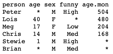
print(family) person age sex funny age.months
1 Peter 42 M High 504
2 Lois 40 F High 480
3 Meg 17 F Low 204
4 Chris 14 M Med 168
5 Stewie 1 M High 12
6 Brian 7 M Med 84Logical Record Subsets
We saw how to use logical flag vectors to subset vectors
We can use logical flag vectors to subset data frames as well
Suppose to have data frame
my_datacontaining a variablemy_variableWant to subset records in
my_datafor whichmy_variablesatisfies a conditionUse commands
flag <- condition(my_data$my_variable)my_data[flag, ]
Example
- Consider again the Family Guy data frame
family - We subset Female characters using flag
family$sex == "F"
[1] FALSE TRUE TRUE FALSE FALSE FALSE# Subset data frame "family" and store in data frame "subset"
subset <- family[flag, ]
print(subset) person age sex funny age.months
2 Lois 40 F High 480
3 Meg 17 F Low 204Part 5:
Data Entry
Reading data from files
R has a many functions for reading characters from stored files
We will see how to read Table-Format files
Table-Formats are just tables stored in plain-text files
Typical file estensions are:
.txtfor plain-text files.csvfor comma-separated values
Table-Formats can be read into R with the command
read.table()
Table-Formats
4 key features
- Header: Used to name columns
- Header should be first line
- Header is optional
- If header present, need to tell R when importing
- If not, R cannot tell if first line is header or data
- Delimiter: Character used to separate entries in each line
- Delimiter character cannot be used for anything else in the file
- Default delimiter is whitespace
Table-Formats
4 key features
- Missing value: Character string used exclusively to denote a missing value
- When reading the file, R will turn these entries into
NA
- When reading the file, R will turn these entries into
- Comments:
- Table files can include comments
- Comment lines start with \quad
# - R ignores such comments
Example
- Table-Format for Family Guy characters can be downloaded here family_guy.txt
- The text file looks like this
- Remarks:
- Header is present
- Delimiter is whitespace
- Missing values denoted by
*
read.table command
Table-Formats can be read via read.table()
Reads
.txtor.csvfilesoutputs a data frame
Options of read.table()
header = T/F- Tells R if a header is present
na.strings = "string"- Tells R that
"string"meansNA(missing values)
- Tells R that
Reading our first Table-Format file
To read family_guy.txt into R proceed as follows:
Download family_guy.txt and move file to Desktop
Open the R Console and change working directory to Desktop
- Read
family_guy.txtinto R and store it in data framefamilywith code
- Note that we are telling
read.table()thatfamily_guy.txthas a header- Missing values are denoted by
*
- Print data frame
familyto screen
  person age sex funny age.mon
1  Peter  NA   M  High     504
2   Lois  40   F  <NA>     480
3    Meg  17   F   Low     204
4  Chris  14   M   Med     168
5 Stewie   1   M  High      NA
6 Brian NA M Med NA- For comparison this is the
.txtfile
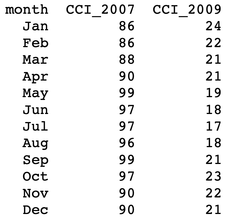
Example: t-test
Data: Analysis of Consumer Confidence Index for 2008 crisis (seen in Lecture 3)
- We imported data into R using
c() - This is ok for small datasets
- Suppose the CCI data is stored in a
.txtfile instead
Goal: Perform t-test on CCI difference for mean difference \mu = 0
- By reading CCI data into R using
read.table() - By manipulating CCI data using data frames
The CCI dataset can be downloaded here 2008_crisis.txt
The text file looks like this
To perform the t-test on data 2008_crisis.txt we proceed as follows:
Download dataset 2008_crisis.txt and move file to Desktop
Open the R Console and change working directory to Desktop
- Read
2008_crisis.txtinto R and store it in data framescoreswith code
- Store 2nd and 3rd columns of
scoresinto 2 vectors
# CCI from 2007 is stored in 2nd column
score_2007 <- scores[, 2]

# CCI from 2009 is stored in 3nd column
score_2009 <- scores[, 3]- From here, the t-test can be performed as done in Lecture 3
# Compute vector of differences
difference <- score_2007 - score_2009

# Perform t-test on difference with null hypothesis mu = 0
t.test(difference, mu = 0)$p.value
[1] 4.860686e-13- We obtain the same result of Lecture 3
- p-value is p < 0.05 \implies Reject H_0: The mean difference is not 0
- For convenience, you can download the full code 2008_crisis_code.R
Part 6:
Least squares
Example: Blood Pressure
10 patients treated with both Drug A and Drug B
- These drugs cause change in blood pressure
- Patients are given the drugs one at a time
- Changes in blood pressure are recorded
- For patient i we denote by
- x_i the change caused by Drug A
- y_i the change caused by Drug B
| i | x_i | y_i |
|---|---|---|
| 1 | 1.9 | 0.7 |
| 2 | 0.8 | -1.0 |
| 3 | 1.1 | -0.2 |
| 4 | 0.1 | -1.2 |
| 5 | -0.1 | -0.1 |
| 6 | 4.4 | 3.4 |
| 7 | 4.6 | 0.0 |
| 8 | 1.6 | 0.8 |
| 9 | 5.5 | 3.7 |
| 10 | 3.4 | 2.0 |
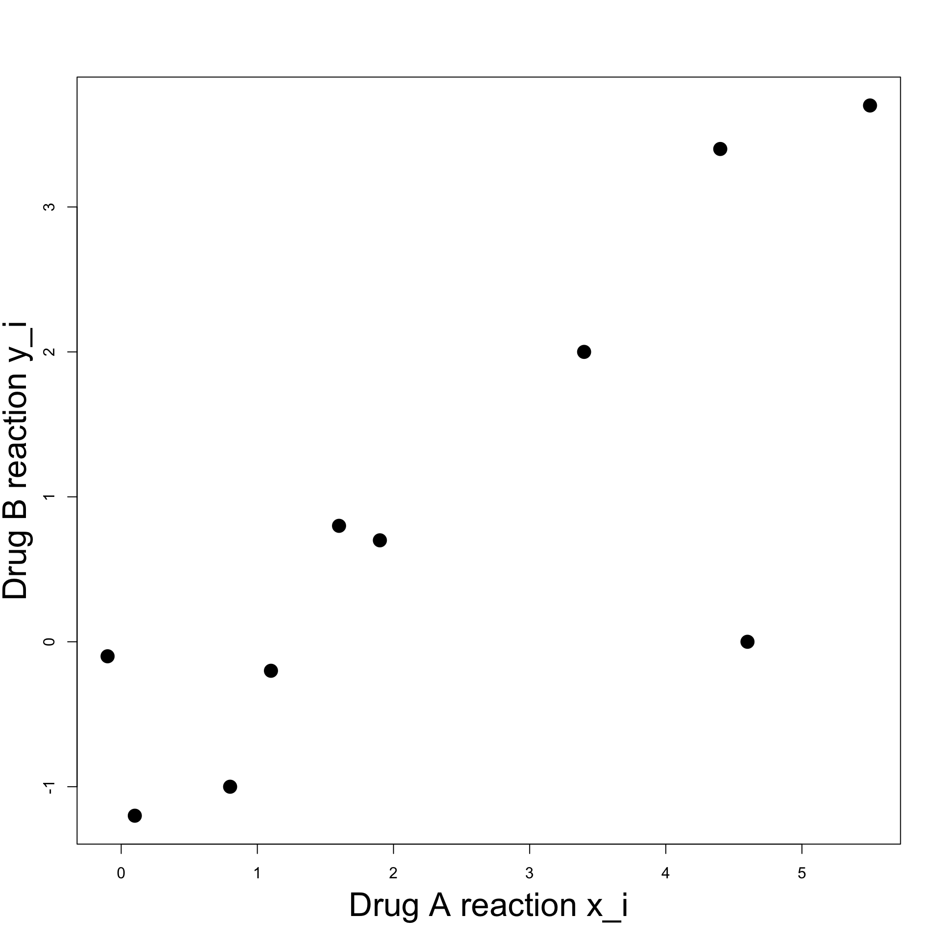
Example: Blood Pressure
Goal:
- Predict reaction to Drug B, knowing reaction to Drug A
- This means predict y_i from x_i
Plot:
- To visualize data we can plot pairs (x_i,y_i)
- Points seem to align
- It seems there is a linear relation between x_i and y_i
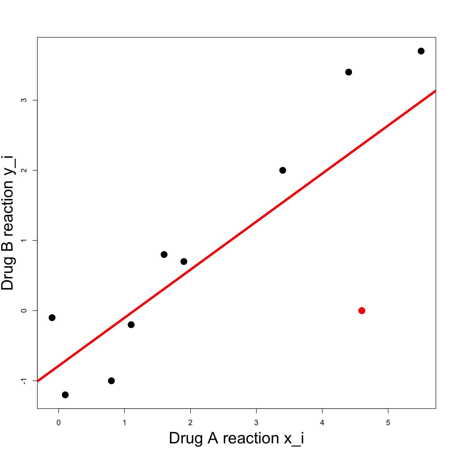
Example: Blood Pressure
Linear relation:
Try to fit a line through the data
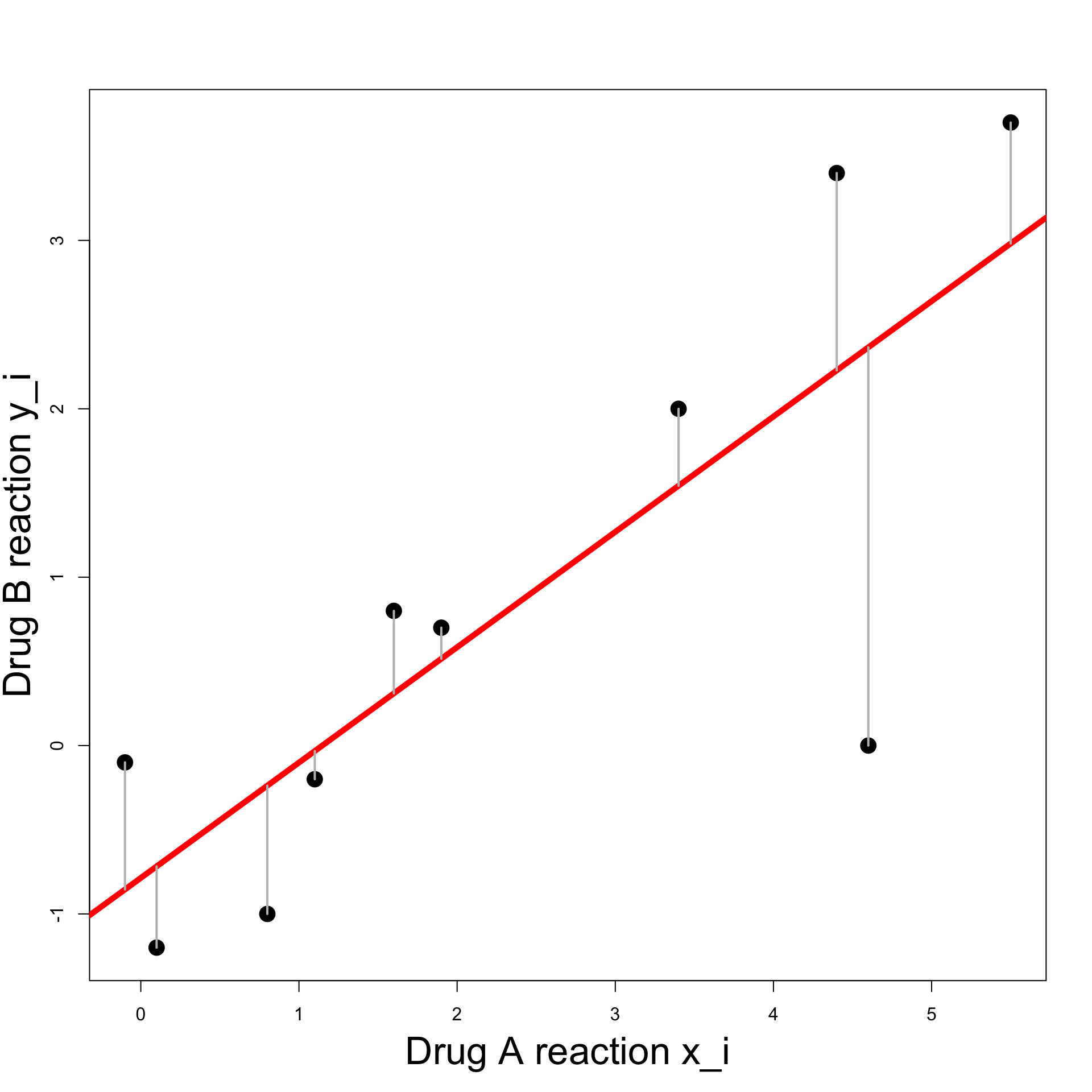
Line roughly predicts y_i from x_i
However note the outlier (x_7,y_7) = (4.6, 0) (red point)
How is such line constructed?
Example: Blood Pressure
Least Squares Line:
- A general line has equation
y = \beta x + \alpha
for some
- slope \beta
- intercept \alpha
- Value predicted by the line for x_i is \hat{y}_i = \beta x_i + \alpha
Example: Blood Pressure
Least Squares Line:
We would like predicted and actual value to be close \hat{y}_i \approx y_i
Hence the vertical difference has to be small y_i - \hat{y}_i \approx 0

Example: Blood Pressure
Least Squares Line:
We want \hat{y}_i - y_i \approx 0 \,, \qquad \forall \, i
Can be achieved by minimizing the sum of squares \min_{\alpha, \beta} \ \sum_{i} \ (y_i - \hat{y}_i)^2 \hat{y}_i = \beta x_i + \alpha

Residual Sum of Squares
Definition
Let (x_1,y_1), \ldots, (x_n, y_n) be a set of n pair of points. Consider the line
y = \beta x + \alpha
The Residual Sum of Squares associated to the line is
\mathop{\mathrm{RSS}}(\alpha,\beta) := \sum_{i=1}^n (y_i-\alpha-{\beta}x_i)^2
Note: \mathop{\mathrm{RSS}} can be seen as a function \mathop{\mathrm{RSS}}\colon \mathbb{R}^2 \to \mathbb{R}\qquad \quad \mathop{\mathrm{RSS}}= \mathop{\mathrm{RSS}}(\alpha,\beta)
\mathop{\mathrm{RSS}}(\alpha,\beta) for Blood Pressure data
Summary statistics
For a given sample (x_1,y_1), \ldots, (x_n, y_n), define
Sample Means: \overline{x} := \frac{1}{n} \sum_{i=1}^n x_i \qquad \quad \overline{y} := \frac{1}{n} \sum_{i=1}^n y_i
Sums of squares: S_{xx} := \sum_{i=1}^n ( x_i - \overline{x} )^2 \qquad \quad S_{yy} := \sum_{i=1}^n ( y_i - \overline{y} )^2
Sum of cross-products: S_{xy} := \sum_{i=1}^n ( x_i - \overline{x} ) ( y_i - \overline{y} )
Minimizing the RSS
Theorem
Given (x_1,y_1), \ldots, (x_n, y_n), consider the minimization problem \begin{equation} \tag{M} \min_{\alpha,\beta } \ \mathop{\mathrm{RSS}}= \min_{\alpha,\beta} \ \sum_{i=1}^n (y_i-\alpha-{\beta}x_i)^2 \end{equation} Then
- There exists a unique line solving (M)
- Such line has the form y = \hat{\beta} x + \hat{\alpha} with \hat{\beta} = \frac{S_{xy}}{S_{xx}} \qquad \qquad \hat{\alpha} = \overline{y} - \hat{\beta} \ \overline{x}
Positive semi-definite matrix
To prove the Theorem we need some background results
A symmetric matrix is positive semi-definite if all the eigenvalues \lambda_i satisfy \lambda_i \geq 0
Proposition: A 2 \times 2 symmetric matrix M is positive semi-definite iff \det M \geq 0 \,, \qquad \quad \operatorname{Tr}(M) \geq 0
Positive semi-definite Hessian
- Suppose given a smooth function of 2 variables
f \colon \mathbb{R}^2 \to \mathbb{R}\qquad \quad f = f (x,y)
- The Hessian of f is the matrix
\nabla^2 f = \left( \begin{array}{cc} f_{xx} & f_{xy} \\ f_{yx} & f_{yy} \\ \end{array} \right)
Positive semi-definite Hessian
- In particular the Hessian is positive semi-definite iff
\det \nabla^2 f = f_{xx} f_{yy} - f_{xy}^2 \geq 0 \qquad \quad f_{xx} + f_{yy} \geq 0
- Side Note: For C^2 functions it holds that
\nabla^2 f \, \text{ is positive semi-definite} \qquad \iff \qquad f \, \text{ is convex}
Optimality conditions
Lemma
Suppose f \colon \mathbb{R}^2 \to \mathbb{R} has positive semi-definite Hessian. They are equivalent
The point (\hat{x},\hat{y}) is a minimizer of f, that is, f(\hat{x}, \hat{y}) = \min_{x,y} \ f(x,y)
The point (\hat{x},\hat{y}) satisfies the optimality conditions \nabla f (\hat{x},\hat{y}) = 0
Note: The proof of the above Lemma can be found in [1]
Example
- The main example of strictly convex function in 2D is
f(x,y) = x^2 + y^2
It is clear that \min_{x,y} \ f(x,y) = \min_{x,y} \ x^2 + y^2 = 0 \,, with the only minimizer being (0,0)
However, let us use the Lemma to prove this fact
- The gradient of f = x^2 + y^2 is
\nabla f = (f_x,f_y) = (2x, 2y)
- Therefore the optimality condition has unique solution
\nabla f = 0 \qquad \iff \qquad x = y = 0
- The Hessian of f is
\nabla^2 f = \left( \begin{array}{cc} f_{xx} & f_{xy} \\ f_{yx} & f_{yy} \end{array} \right) = \left( \begin{array}{cc} 2 & 0 \\ 0 & 2 \end{array} \right)
- The Hessian is positive semi-definite since
\det (\nabla^2) f = 4 > 0 \qquad \qquad \operatorname{Tr}(\nabla^2 f) = 4 > 0
- By the Lemma, we conclude that (0,0) is the unique minimizer of f, that is,
0 = f(0,0) = \min_{x,y} \ f(x,y)
Minimizing the RSS
Proof of Theorem
We go back to proving the RSS Minimization Theorem
Suppose given data points (x_1,y_1), \ldots, (x_n, y_n)
We want to solve the minimization problem
\begin{equation} \tag{M} \min_{\alpha,\beta } \ \mathop{\mathrm{RSS}}= \min_{\alpha,\beta} \ \sum_{i=1}^n (y_i-\alpha-{\beta}x_i)^2 \end{equation}
- In order to use the Lemma we need to compute
\nabla \mathop{\mathrm{RSS}}\quad \text{ and } \quad \nabla^2 \mathop{\mathrm{RSS}}
Minimizing the RSS
Proof of Theorem
We first compute \nabla \mathop{\mathrm{RSS}} and solve the optimality conditions \nabla \mathop{\mathrm{RSS}}(\alpha,\beta) = 0
To this end, recall that \overline{x} := \frac{\sum_{i=1}^nx_i}{n} \qquad \implies \qquad \sum_{i=1}^n x_i = n \overline{x}
Similarly, we have \sum_{i=1}^n y_i = n \overline{y}
Minimizing the RSS
Proof of Theorem
- Therefore we get
\begin{align*} \mathop{\mathrm{RSS}}_{\alpha} & = -2\sum_{i=1}^n(y_i- \alpha- \beta x_i) \\[10pt] & = - 2 n \overline{y} + 2n \alpha + 2 \beta n \overline{x} \\[20pt] \mathop{\mathrm{RSS}}_{\beta} & = -2\sum_{i=1}^n x_i (y_i- \alpha - \beta x_i) \\[10pt] & = - 2 \sum_{i=1}^n x_i y_i + 2 \alpha n \overline{x} + 2 \beta \sum_{i=1}^n x_i^2 \end{align*}
Minimizing the RSS
Proof of Theorem
- Hence the optimality conditions are
\begin{align} - 2 n \overline{y} + 2n \alpha + 2 \beta n \overline{x} & = 0 \tag{1} \\[20pt] - 2 \sum_{i=1}^n x_i y_i + 2 \alpha n \overline{x} + 2 \beta \sum_{i=1}^n x_i^2 & = 0 \tag{2} \end{align}
Minimizing the RSS
Proof of Theorem
- Equation (1) is
-2 n \overline{y} + 2n \alpha + 2 \beta n \overline{x} = 0
- By simplifying and rearraging, we find that (1) is equivalent to
\alpha = \overline{y}- \beta \overline{x}
Minimizing the RSS
Proof of Theorem
- Equation (2) is equivalent to
\sum_{i=1}^n x_i y_i - \alpha n \overline{x} - \beta \sum_{i=1}^n x^2_i = 0
- From the previous slide we have \alpha = \overline{y}- \beta \overline{x}
Minimizing the RSS
Proof of Theorem
- Substituting in Equation (2) we get \begin{align*} 0 & = \sum_{i=1}^n x_i y_i - \alpha n \overline{x} - \beta \sum_{i=1}^n x^2_i \\ & = \sum_{i=1}^n x_i y_i - n \overline{x} \, \overline{y} + \beta n \overline{x}^2 - \beta \sum_{i=1}^n x^2_i \\ & = \sum_{i=1}^n (x_i y_i - \overline{x} \, \overline{y} ) - \beta \left( \sum_{i=1}^n x^2_i - n\overline{x}^2 \right) = S_{xy} - \beta S_{xx} \end{align*} where we used the usual identity S_{xx} = \sum_{i=1}^n ( x_i - \overline{x})^2 = \sum_{i=1}^n x_i^2 - n\overline{x}^2
Minimizing the RSS
Proof of Theorem
Hence Equation (2) is equivalent to \beta = \frac{S_{xy}}{ S_{xx} }
Also recall that Equation (1) is equivalent to \alpha = \overline{y}- \beta \overline{x}
Therefore (\hat\alpha, \hat\beta) solves the optimality conditions \nabla \mathop{\mathrm{RSS}}= 0 iff \hat\alpha = \overline{y}- \hat\beta \overline{x} \,, \qquad \quad \hat\beta = \frac{S_{xy}}{ S_{xx} }
Minimizing the RSS
Proof of Theorem
We need to compute \nabla^2 \mathop{\mathrm{RSS}}
To this end recall that \mathop{\mathrm{RSS}}_{\alpha} = - 2 n \overline{y} + 2n \alpha + 2 \beta n \overline{x} \,, \quad \mathop{\mathrm{RSS}}_{\beta} = - 2 \sum_{i=1}^n x_i y_i + 2 \alpha n \overline{x} + 2 \beta \sum_{i=1}^n x_i^2
Therefore we have \begin{align*} \mathop{\mathrm{RSS}}_{\alpha \alpha} & = 2n \qquad & \mathop{\mathrm{RSS}}_{\alpha \beta} & = 2 n \overline{x} \\ \mathop{\mathrm{RSS}}_{\beta \alpha } & = 2 n \overline{x} \qquad & \mathop{\mathrm{RSS}}_{\beta \beta} & = 2 \sum_{i=1}^{n} x_i^2 \end{align*}
Minimizing the RSS
Proof of Theorem
- The Hessian determinant is
\begin{align*} \det (\nabla^2 \mathop{\mathrm{RSS}}) & = \mathop{\mathrm{RSS}}_{\alpha \alpha}\mathop{\mathrm{RSS}}_{\beta \beta} - \mathop{\mathrm{RSS}}_{\alpha \beta}^2 \\[10pt] & = 4n \sum_{i=1}^{n} x_i^2 - 4 n^2 \overline{x}^2 \\[10pt] & = 4n \left( \sum_{i=1}^{n} x_i^2 - n \overline{x}^2 \right) \\[10pt] & = 4n S_{xx} \end{align*}
Minimizing the RSS
Proof of Theorem
- Recall that
S_{xx} = \sum_{i=1}^n (x_i - \overline{x})^2 \geq 0
- Therefore we have
\det (\nabla^2 \mathop{\mathrm{RSS}}) = 4n S_{xx} \geq 0
Minimizing the RSS
Proof of Theorem
- We also have
\operatorname{Tr}(\nabla^2\mathop{\mathrm{RSS}}) = \mathop{\mathrm{RSS}}_{\alpha \alpha} + \mathop{\mathrm{RSS}}_{\beta \beta} = 2n + 2 \sum_{i=1}^{n} x_i^2 \geq 0
Therefore we have proven \det( \nabla^2 \mathop{\mathrm{RSS}}) \geq 0 \,, \qquad \quad \operatorname{Tr}(\nabla^2\mathop{\mathrm{RSS}}) \geq 0
As the Hessian is symmetric, we conclude that \nabla^2 \mathop{\mathrm{RSS}} is positive semi-definite
Minimizing the RSS
Proof of Theorem
By the Lemma, we have that all the solutions (\alpha,\beta) to the optimality conditions \nabla \mathop{\mathrm{RSS}}(\alpha,\beta) = 0 are minimizers
Therefore (\hat \alpha,\hat\beta) with \hat\alpha = \overline{y}- \hat\beta \overline{x} \,, \qquad \quad \hat\beta = \frac{S_{xy}}{ S_{xx} } is a minimizer of \mathop{\mathrm{RSS}}, ending the proof
Least-squares line
The previous Theorem motivates the following definition
Definition
Given (x_1,y_1), \ldots, (x_n, y_n), the least-squares line is
y = \hat\beta x + \hat \alpha
where we define
\hat{\alpha} = \overline{y} - \hat{\beta} \ \overline{x} \qquad \qquad \hat{\beta} = \frac{S_{xy}}{S_{xx}}
Part 7:
Worked Example
Worked Example: Blood Pressure
Computing the least-squares line in R
In R, we want to do the following:
Input the data into vectors x and y
Compute the least-square line coefficients \hat{\alpha} = \overline{y} - \hat{\beta} \ \overline{x} \qquad \qquad \hat{\beta} = \frac{S_{xy}}{S_{xx}}
Plot the data points (x_i,y_i)
Overlay the least squares line
| i | x_i | y_i |
|---|---|---|
| 1 | 1.9 | 0.7 |
| 2 | 0.8 | -1.0 |
| 3 | 1.1 | -0.2 |
| 4 | 0.1 | -1.2 |
| 5 | -0.1 | -0.1 |
| 6 | 4.4 | 3.4 |
| 7 | 4.6 | 0.0 |
| 8 | 1.6 | 0.8 |
| 9 | 5.5 | 3.7 |
| 10 | 3.4 | 2.0 |
First Solution
We give a first solution using elementary R functions
The code to input the data into a data-frame is as follows
# Input blood pressure changes data into data-frame

changes <- data.frame(drug_A = c(1.9, 0.8, 1.1, 0.1, -0.1,
                                 4.4, 4.6, 1.6, 5.5, 3.4),
                      drug_B = c(0.7, -1.0, -0.2, -1.2, -0.1,
                                 3.4, 0.0, 0.8, 3.7, 2.0)
)- To shorten the code we assign
drug_Aanddrug_Bto vectorsxandy
- Compute averages \overline{x}, \overline{y} and covariances S_{xx}, S_{xy}
- Compute the least-square line coefficients \hat{\beta} = \frac{S_{xy}}{S_{xx}} \,, \qquad \qquad \hat{\alpha} = \overline{y} - \hat{\beta} \ \overline{x}
# Compute least-square line coefficients
beta <- S_xy / S_xx
alpha <- ybar - beta * xbar

# Print coefficients
cat("\nCoefficient alpha =", alpha)
cat("\nCoefficient beta =", beta)
Coefficient alpha = -0.7861478
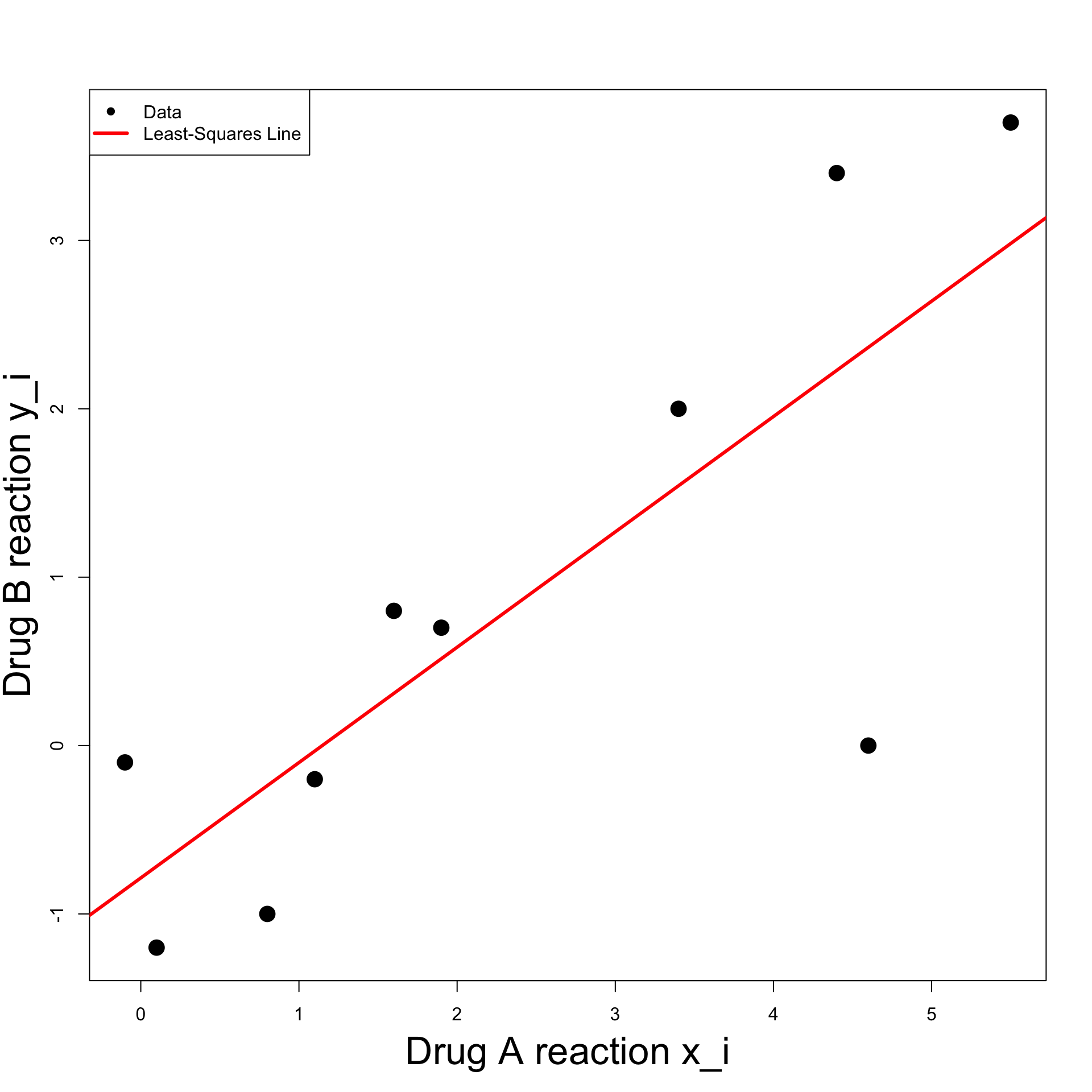
Coefficient beta = 0.685042- Plot the data pairs (x_i,y_i)
# Plot the data
plot(x, y, xlab = "", ylab = "", pch = 16, cex = 2)

# Add labels
mtext("Drug A reaction x_i", side = 1, line = 3, cex = 2.1)
mtext("Drug B reaction y_i", side = 2, line = 2.5, cex = 2.1)
Note: We have added a few cosmetic options
pch = 16plots points with black circlescex = 2stands for character expansion – Specifies width of pointsmtextis used to fine-tune the axis labelsside = 1stands for x-axisside = 2stands for y-axislinespecifies distance of label from axis
- To plot a line y = bx + a
abline(a, b)
- Overlay the least squares line y = \hat{\beta}x + \hat{\alpha}
- Note: Cosmetic options
colspecifies color of the plotlwdspecifies line width
- For clarity, we can add legend to plot
The code can be downloaded here least_squares_1.R
Running the code we obtain the plot below
Second Solution
- The second solution uses the R function
lm lmstands for linear model- First we input the data into a data-frame
- Use
lmto fit the least-squares linelm(formula, data)dataexpects a data-frame in inputformulastands for the relation to fit
- In the case of least-squares:
formula = y ~ xxandyare names of two variables in the data-frame- Symbol
y ~ xcan be read as: y modelled as function of x
Note: Storing data in data-frame is optional
We can just store data in vectors
xandyThen fit the least-squares line with
lm(y ~ x)
- The command to fit the least-squares line on
changesis
# Fit least squares line
least_squares <- lm(formula = drug_B ~ drug_A, data = changes)

# Print output
print(least_squares)
Call:
lm(formula = drug_B ~ drug_A, data = changes)

Coefficients:
(Intercept)       drug_A
    -0.7861       0.6850
- The above tells us that the estimators are
\hat \alpha = -0.7861 \,, \qquad \quad \hat \beta = 0.6850
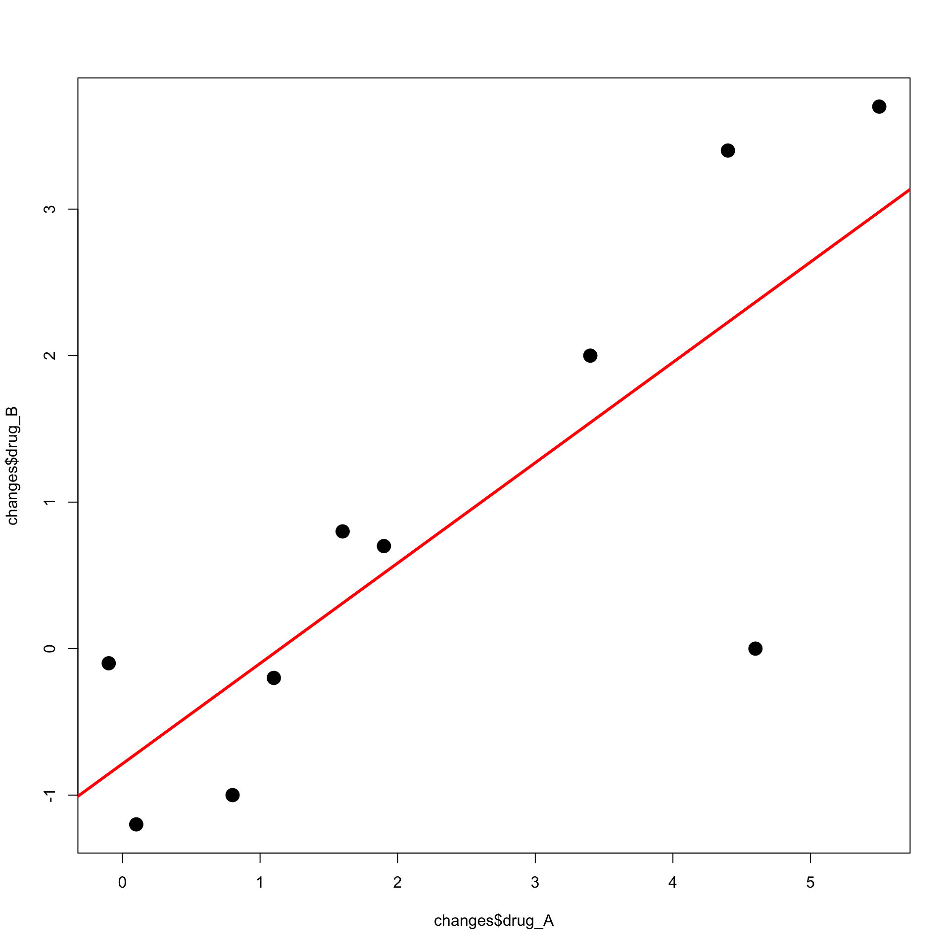
- We can now plot the data with the following command
- 1st coordinate is the vector
changes$drug_A - 2nd coordinate is the vector
changes$drug_B
- 1st coordinate is the vector
The least-squares line is currently stored in
least_squaresTo add the line to the current plot use
abline
The code can be downloaded here least_squares_2.R
Running the code we obtain the plot below
References
[1]
Fusco, Nicola, Marcellini, Paolo, Sbordone, Carlo, Mathematical analysis: Functions of several real variables and applications, Springer, 2022.