Statistical Models

Lecture 4

Dr. Silvio Fanzon

S.Fanzon@hull.ac.uk

University of Hull

Lecture 4:
Two-sample
hypothesis tests

Outline of Lecture 4

1. Two-sample hypothesis tests
2. Two-sample t-test
3. Two-sample t-test: Example
4. The Welch t-test
5. The t-test for paired samples
6. The F-distribution
7. Two-sample F-test
8. Worked Example

Part 4:
Two-sample
hypothesis tests

Overview

In Lecture 3:

• We looked at data on CCI before and after the 2008 crash
• In this case data for each month is directly comparable
• Can then construct the difference between the 2007 and 2009 values
• Analysis reduces from a two-sample to a one-sample problem

Question

How do we analyze two samples that cannot be paired?

Problem statement

Goal: compare mean and variance of 2 independent normal samples

• First sample:
  • X_1, \ldots, X_n from normal population N(\mu_X,\sigma_X^2)
• Second sample:
  • Y_1, \ldots, Y_m from normal population N(\mu_Y,\sigma_Y^2)
• We may have n \neq m
  • Samples cannot be paired due to different size!

Tests available:

• Two-sample t-test to test for difference in means
• Two-sample F-test to test for difference in variances (next week)

Why is this important?

• Hypothesis testing starts to get interesting with 2 or more samples

• t-test and F-test show the normal distribution family in action

• This is also the maths behind regression

  • Same methods apply to seemingly unrelated problems
  • Regression is a big subject in statistics

Normal distribution family in action

Two-sample t-test

• Want to compare the means of two independent samples
• At the same time population variances are unknown
• Therefore both variances are estimated with sample variances
• Test statistic is t_k-distributed with k linked to the total number of observations

Normal distribution family in action

Two-sample F-test

• Want to compare the variance of two independent samples

• This can be done by studying the ratio of the sample variances S^2_X/S^2_Y

• We have already shown that \frac{(n - 1) S^2_X}{\sigma^2_X} \sim \chi^2_{n - 1} \qquad \frac{(m - 1) S^2_Y}{\sigma^2_Y} \sim \chi^2_{m - 1}

Normal distribution family in action

Two-sample F-test

• Hence we can study statistic F = \frac{S^2_X / \sigma_X^2}{S^2_Y / \sigma_Y^2}

• We will see that F has F-distribution (next week)

Part 5:
Two-sample t-test

The two-sample t-test

Assumptions: Suppose given samples from 2 independent normal populations

• X_1, \ldots ,X_n iid with distribution N(\mu_X,\sigma_X^2)
• Y_1, \ldots ,Y_m iid with distribution N(\mu_Y,\sigma_Y^2)

Further assumptions:

• In general n \neq m, so that one-sample t-test cannot be applied
• The two populations have same variance \sigma^2_X = \sigma^2_Y = \sigma^2

Note: Assuming same variance is simplification. Removing it leads to Welch t-test

The two-sample t-test

Goal: Compare means \mu_X and \mu_Y

Hypothesis set: We test for a difference in means H_0 \colon \mu_X = \mu_Y \qquad H_1 \colon \mu_X \neq \mu_Y

t-statistic: The general form is T = \frac{\text{Estimate}-\text{Hypothesised value}}{\text{e.s.e.}}

The two-sample t-statistic

• Define the sample means \overline{X} = \frac{1}{n} \sum_{i=1}^n X_i \qquad \qquad \overline{Y} = \frac{1}{m} \sum_{i=1}^m Y_i

• Notice that {\rm I\kern-.3em E}[ \overline{X} ] = \mu_X \qquad \qquad {\rm I\kern-.3em E}[ \overline{Y} ] = \mu_Y

• Therefore we can estimate \mu_X - \mu_Y with the sample means, that is, \text{Estimate} = \overline{X} - \overline{Y}

The two-sample t-statistic

• Since we are testing for difference in mean, we have \text{Hypothesised value} = \mu_X - \mu_Y

• The Estimated Standard Error is the standard deviation of estimator \text{e.s.e.} = \text{Standard Deviation of } \overline{X} -\overline{Y}

The two-sample t-statistic

• Therefore the two-sample t-statistic is T = \frac{\overline{X} - \overline{Y} - (\mu_X - \mu_Y)}{\text{e.s.e.}}

• Under the Null Hypothesis that \mu_X = \mu_Y, the t-statistic becomes T = \frac{\overline{X} - \overline{Y} }{\text{e.s.e.}}

A note on the degrees of freedom (df)

• The general rule is \text{df} = \text{Sample size} - \text{No. of estimated parameters}

• Sample size in two-sample t-test:

  • n in the first sample
  • m in the second sample
  • Hence total number of observations is n + m

• No. of estimated parameters is 2: Namely \mu_X and \mu_Y

• Hence degree of freedoms in two-sample t-test is {\rm df} = n + m - 2 (more on this later)

The estimated standard error

• Recall: We are assuming populations have same variance \sigma^2_X = \sigma^2_Y = \sigma^2

• We need to compute the estimated standard error \text{e.s.e.} = \text{Standard Deviation of } \ \overline{X} -\overline{Y}

• Variance of sample mean was computed in the Lemma in Slide 72 Lecture 2

• Since \overline{X} \sim N(\mu_X,\sigma^2) and \overline{Y} \sim N(\mu_Y,\sigma^2), by the Lemma we get {\rm Var}[\overline{X}] = \frac{\sigma^2}{n} \,, \qquad \quad {\rm Var}[\overline{Y}] = \frac{\sigma^2}{m}

The estimated standard error

• Since X_i and Y_i are independent we get {\rm Cov}(X_i,Y_j)=0

• By bilinearity of covariance we infer {\rm Cov}( \overline{X} , \overline{Y} ) = \frac{1}{n \cdot m} \sum_{i=1}^n \sum_{j=1}^m {\rm Cov}(X_i,Y_j) = 0

• We can then compute \begin{align*} {\rm Var}[ \overline{X} - \overline{Y} ] & = {\rm Var}[ \overline{X} ] + {\rm Var}[ \overline{Y} ] - 2 {\rm Cov}( \overline{X} , \overline{Y} ) \\ & = {\rm Var}[ \overline{X} ] + {\rm Var}[ \overline{Y} ] \\ & = \sigma^2 \left( \frac{1}{n} + \frac{1}{m} \right) \end{align*}

The estimated standard error

• Taking the square root gives \text{S.D.}(\overline{X} - \overline{Y} )= \sigma \ \sqrt{\frac{1}{n}+\frac{1}{m}}

• Therefore, the t-statistic is T = \frac{\overline{X} - \overline{Y} - (\mu_X - \mu_Y)}{\text{e.s.e.}} = \frac{\overline{X} - \overline{Y} - (\mu_X - \mu_Y)}{\sigma \ \sqrt{\dfrac{1}{n}+\dfrac{1}{m}}}

Estimating the variance

The t-statistic is currently T = \frac{\overline{X} - \overline{Y} - (\mu_X - \mu_Y)}{\sigma \ \sqrt{\dfrac{1}{n}+\dfrac{1}{m}}}

• Variance \sigma^2 is unknown: we need to estimate it!

• Define the sample variances

S_X^2 = \frac{ \sum_{i=1}^n X_i^2 - n \overline{X}^2 }{n-1} \qquad \qquad S_Y^2 = \frac{ \sum_{i=1}^m Y_i^2 - m \overline{Y}^2 }{m-1}

Estimating the variance

• Recall that X_1, \ldots , X_n \sim N(\mu_X, \sigma^2) \qquad \qquad Y_1, \ldots , Y_m \sim N(\mu_Y, \sigma^2)

• From Lecture 2, we know that S_X^2 and S_Y^2 are unbiased estimators of \sigma^2, i.e. {\rm I\kern-.3em E}[ S_X^2 ] = {\rm I\kern-.3em E}[ S_Y^2 ] = \sigma^2

• Therefore, both S_X^2 and S_Y^2 can be used to estimate \sigma^2

Estimating the variance

• We can improve the estimate of \sigma^2 by combining S_X^2 and S_Y^2

• We will consider a (convex) linear combination S^2 := \lambda_X S_X^2 + \lambda_Y S_Y^2 \,, \qquad \lambda_X + \lambda_Y = 1

• S^2 is still an unbiased estimator of \sigma^2, since \begin{align*} {\rm I\kern-.3em E}[S^2] & = {\rm I\kern-.3em E}[ \lambda_X S_X^2 + \lambda_Y S_Y^2 ] \\ & = \lambda_X {\rm I\kern-.3em E}[S_X^2] + \lambda_Y {\rm I\kern-.3em E}[S_Y^2] \\ & = (\lambda_X + \lambda_Y) \sigma^2 \\ & = \sigma^2 \end{align*}

Estimating the variance

We choose coefficients \lambda_X and \lambda_Y which reflect sample sizes \lambda_X := \frac{n - 1}{n + m - 2} \qquad \qquad \lambda_Y := \frac{m - 1}{n + m - 2}

Notes:

• We have \lambda_X + \lambda_Y = 1

• Denominators in \lambda_X and \lambda_Y are degrees of freedom {\rm df } = n + m - 2

• This choice is made so that S^2 has chi-squared distribution (more on this later)

Pooled estimator of variance

Definition

The pooled estimator of \sigma^2 is defined as S_p^2 := \lambda_X S_X^2 + \lambda_Y S_Y^2 = \frac{(n-1) S_X^2 + (m-1) S_Y^2}{n + m - 2}

Note:

• n=m implies \lambda_X = \lambda_Y
• In this case S_X^2 and S_Y^2 have same weight in S_p^2

The two-sample t-statistic

• The t-statistic has currently the form T = \frac{\overline{X} - \overline{Y} - (\mu_X - \mu_Y)}{\sigma \ \sqrt{\dfrac{1}{n}+\dfrac{1}{m}}}

• We replace \sigma with the pooled estimator S_p

The two-sample t-statistic

Definition

The two sample t-statistic is defined as T := \frac{\overline{X} - \overline{Y} - (\mu_X - \mu_Y)}{ S_p \ \sqrt{\dfrac{1}{n}+\dfrac{1}{m}}}

Note: Under the Null Hypothesis that \mu_X = \mu_Y this becomes T = \frac{\overline{X} - \overline{Y}}{ S_p \ \sqrt{\dfrac{1}{n}+\dfrac{1}{m}}} = \frac{\overline{X} - \overline{Y}}{ \sqrt{ \dfrac{ (n-1) S_X^2 + (m-1) S_Y^2 }{n + m - 2} } \ \sqrt{\dfrac{1}{n}+\dfrac{1}{m}}}

Distribution of two-sample t-statistic

Theorem

The two sample t-statistic has t_{n+m-2} distribution T := \frac{\overline{X} - \overline{Y} - (\mu_X - \mu_Y)}{ S_p \ \sqrt{\dfrac{1}{n}+\dfrac{1}{m}}} \sim t_{n + m - 2}

Distribution of two-sample t-statistic

Proof

• We have already seen that \overline{X} - \overline{Y} is normal with {\rm I\kern-.3em E}[\overline{X} - \overline{Y}] = \mu_X - \mu_Y \qquad \qquad {\rm Var}[\overline{X} - \overline{Y}] = \sigma^2 \left( \frac{1}{n} + \frac{1}{m} \right)

• Therefore we can rescale \overline{X} - \overline{Y} to get U := \frac{\overline{X} - \overline{Y} - (\mu_X - \mu_Y)}{ \sigma \sqrt{ \dfrac{1}{n} + \dfrac{1}{m}}} \sim N(0,1)

Distribution of two-sample t-statistic

Proof

• We are assuming X_1, \ldots, X_n iid N(\mu_X,\sigma^2)

• Therefore, as already shown, we have \frac{ (n-1) S_X^2 }{ \sigma^2 } \sim \chi_{n-1}^2

• Similarly, since Y_1, \ldots, Y_m iid N(\mu_Y,\sigma^2), we get \frac{ (m-1) S_Y^2 }{ \sigma^2 } \sim \chi_{m-1}^2

Distribution of two-sample t-statistic

Proof

• Since X_i and Y_j are independent, we also have that \frac{ (n-1) S_X^2 }{ \sigma^2 } \quad \text{ and } \quad \frac{ (m-1) S_Y^2 }{ \sigma^2 } \quad \text{ are independent}

• In particular we obtain \frac{ (n-1) S_X^2 }{ \sigma^2 } + \frac{ (m-1) S_Y^2 }{ \sigma^2 } \sim \chi_{n-1}^2 + \chi_{m-1}^2 \sim \chi_{m + n- 2}^2

Distribution of two-sample t-statistic

Proof

• Recall the definition of S_p^2 S_p^2 = \frac{(n-1) S_X^2 + (m-1) S_Y^2}{ n + m - 2 }

• Therefore V := \frac{ (n+m-2) S_p^2 }{ \sigma^2 } = \frac{ (n - 1) S_X^2}{ \sigma^2} + \frac{ (m-1) S_Y^2 }{ \sigma^2 } \sim \chi_{n + m - 2}^2

Distribution of two-sample t-statistic

Proof

• Rewrite T as \begin{align*} T & = \frac{\overline{X} - \overline{Y} - (\mu_X - \mu_Y)}{ S_p \ \sqrt{\dfrac{1}{n}+\dfrac{1}{m}}} \\ & = \frac{\overline{X} - \overline{Y} - (\mu_X - \mu_Y)}{ \sigma \sqrt{ \dfrac{1}{n} + \dfrac{1}{m} } } \Bigg/ \sqrt{ \frac{ (n + m - 2) S_p^2 \big/ \sigma^2}{ (n+ m - 2) } } \\ & = \frac{U}{\sqrt{V/(n+m-2)}} \end{align*}

Distribution of two-sample t-statistic

Proof

• By construction \overline{X}- \overline{Y} is independent of S_X^2 and S_Y^2

• Therefore \overline{X}- \overline{Y} is independent of S_p^2

• We conclude that U and V are independent

• In conclusion, we have shown that T = \frac{U}{\sqrt{V/(n+m-2)}} \,, \qquad U \sim N(0,1) \,, \qquad V \sim \chi_{n + m - 2}^2

• By the Theorem in Slide 118 of Lecture 2, we conclude that T \sim t_{n+m-2}

The two-sample t-test

Suppose given two independent samples

• Sample x_1, \ldots, x_n from N(\mu_X,\sigma^2) of size n
• Sample y_1, \ldots, y_m from N(\mu_Y,\sigma^2) of size m

The two-sided hypothesis for difference in means is H_0 \colon \mu_X = \mu_Y \,, \quad \qquad H_1 \colon \mu_X \neq \mu_Y

The one-sided alternative hypotheses are H_1 \colon \mu_X < \mu_Y \quad \text{ or } \quad H_1 \colon \mu_X > \mu_Y

Procedure: 3 Steps

1. Calculation: Compute the two-sample t-statistic t = \frac{ \overline{x} - \overline{y}}{ s_p \ \sqrt{ \dfrac{1}{n} + \dfrac{1}{m} }} where sample means and pooled variance estimator are \overline{x} = \frac{1}{n} \sum_{i=1}^n x_i \qquad \overline{y} = \frac{1}{m} \sum_{i=1}^m y_i \qquad s_p^2 = \frac{ (n-1) s_X^2 + (m - 1) s_Y^2 }{ m + n - 2} s_X^2 = \frac{\sum_{i=1}^n x_i^2 - n \overline{x}^2}{n-1} \qquad s_Y^2 = \frac{\sum_{i=1}^m y_i^2 - m \overline{y}^2}{m-1}

2. Statistical Tables or R: Find either
   • Critical value t^* in Table 1
   • p-value in R

3. Interpretation: Reject H_0 when either p < 0.05 \qquad \text{ or } \qquad t \in \,\,\text{Rejection Region} \qquad \qquad \qquad \qquad (T \, \sim \, t_{n+m-1})

Alternative	Rejection Region	t^*	p-value
\mu_X \neq \mu_Y	|t| > t^*	t_{n+m-1}(0.025)	2P(T > |t|)
\mu_X < \mu_Y	t < - t^*	t_{n+m-1}(0.05)	P(T < t)
\mu_X > \mu_Y	t > t^*	t_{n+m-1}(0.05)	P(T > t)

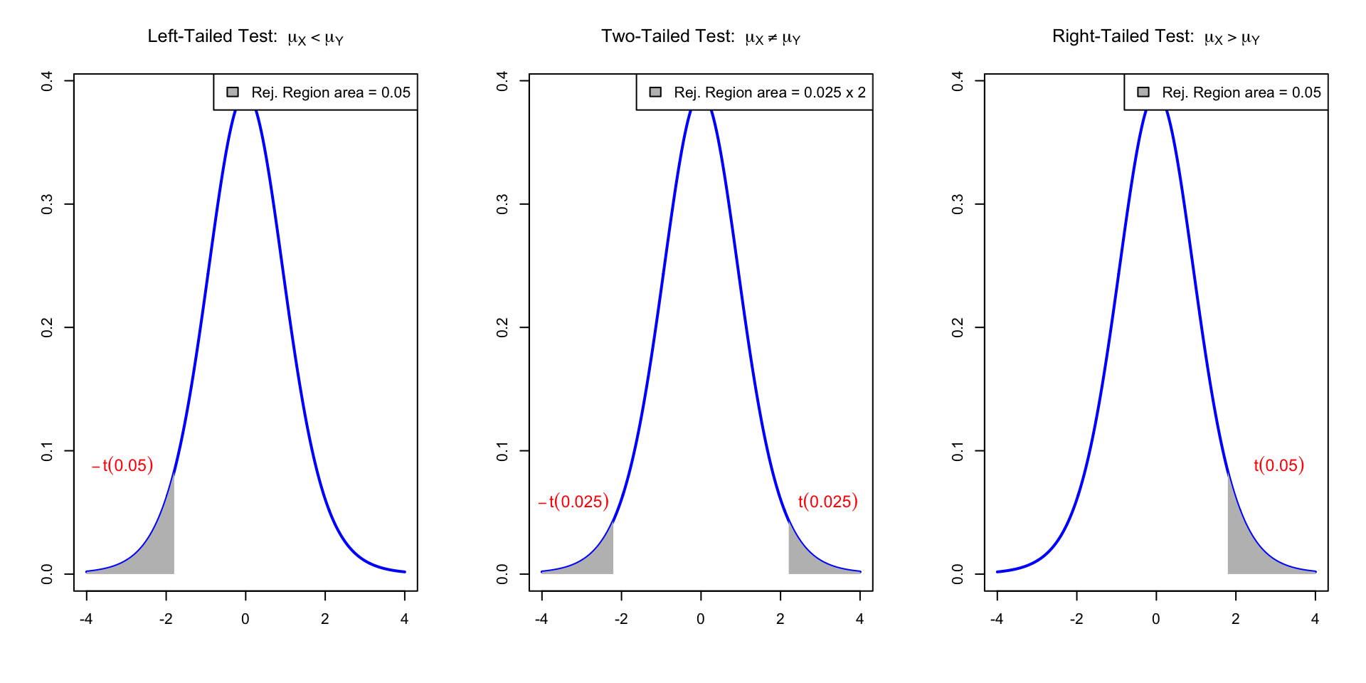
Reject H_0 if t-statistic t falls in the Rejection Region (in gray). Here t \sim t_{n+m-1}

The two-sample t-test in R

General commands

1. Store the samples x_1,\ldots,x_n and y_1,\ldots,y_m in two R vectors
   • x <- c(x1, ..., xn) \qquad y <- c(y1, ..., ym)
2. Perform a two-sample t-test on x and y

Alternative	R command
\mu_X \neq \mu_Y	t.test(x, y, var.equal = T)
\mu_X < \mu_Y	t.test(x, y, var.equal = T, alt = "less")
\mu_X > \mu_Y	t.test(x, y, var.equal = T, alt = "greater")

3. Read output: similar to one-sample t-test
   • The main quantity of interest is p-value

Comments on command t.test(x, y)

1. mu = mu0 tells R to test null hypothesis: H_0 \colon \mu_X - \mu_Y = \mu_0 \qquad \quad (\text{default is } \, \mu_0 = 0)

2. var.equal = T tells R to assume that populations have same variance \sigma_X^2 = \sigma^2_Y

3. In this case R computes the t-statistic with formula discussed earlier t = \frac{ \overline{x} - \overline{y} }{s_p \sqrt{ \dfrac{1}{n} + \dfrac{1}{m} }}

Comments on command t.test(x, y)

Warning: If var.equal = T is not specified then

• R assumes that populations have different variance \sigma_X^2 \neq \sigma^2_Y

• In this case the t-statistic t = \frac{ \overline{x} - \overline{y} }{s_p \sqrt{ \dfrac{1}{n} + \dfrac{1}{m} }} is NOT t-distributed

• R performs the Welch t-test instead of the classic t-test
  (more on this later)

Part 6:
Two-sample t-test
Example

Mathematicians	x_1	x_2	x_3	x_4	x_5	x_6	x_7	x_8	x_9	x_{10}
Wages	36	40	46	54	57	58	59	60	62	63

Accountants	y_1	y_2	y_3	y_4	y_5	y_6	y_7	y_8	y_9	y_{10}	y_{11}	y_{12}	y_{13}
Wages	37	37	42	44	46	48	54	56	59	60	60	64	64

• Samples: Wage data on 10 Mathematicians and 13 Accountants

  • Wages are independent and normally distributed
  • Populations have equal variance

• Quesion: Is there evidence of differences in average pay?

• Answer: Two-sample two-sided t-test for the hypothesis H_0 \colon \mu_X = \mu_Y \,,\qquad H_1 \colon \mu_X \neq \mu_Y

Calculations: First sample

• Sample size: \ n = No. of Mathematicians = 10

• Mean: \bar{x} = \frac{\sum_{i=1}^n x_i}{n} = \frac{36+40+46+ \ldots +62+63}{10}=\frac{535}{10}=53.5

• Variance: \begin{align*} s^2_X & = \frac{\sum_{i=1}^n x_i^2 - n \bar{x}^2}{n -1 } \\ \sum_{i=1}^n x_i^2 & = 36^2+40^2+46^2+ \ldots +62^2+63^2 = 29435 \\ s^2_X & = \frac{29435-10(53.5)^2}{9} = 90.2778 \end{align*}

Calculations: Second sample

• Sample size: \ m = No. of Accountants = 13

• Mean: \bar{y} = \frac{37+37+42+ \dots +64+64}{13} = \frac{671}{13} = 51.6154

• Variance: \begin{align*} s^2_Y & = \frac{\sum_{i=1}^m y_i^2 - m \bar{y}^2}{m - 1} \\ \sum_{i=1}^m y_i^2 & = 37^2+37^2+42^2+ \ldots +64^2+64^2 = 35783 \\ s^2_Y & = \frac{35783-13(51.6154)^2}{12} = 95.7547 \end{align*}

Calculations: Pooled Variance

• Pooled variance: \begin{align*} s_p^2 & = \frac{(n-1) s_X^2 + (m-1) s_Y^2}{ n + m - 2} \\ & = \frac{(9) 90.2778 + (12) 95.7547 }{ 10 + 13 - 2} \\ & = 93.40746 \end{align*}

• Pooled standard deviation: s_p = \sqrt{93.40746} = 9.6648

Calculations: t-statistic

1. Calculation: Compute the two-sample t-statistic

\begin{align*} t & = \frac{\bar{x} - \bar{y} }{s_p \ \sqrt{\dfrac{1}{n}+\dfrac{1}{m}}} \\ & = \frac{53.5 - 51.6154}{9.6648 \times \sqrt{\dfrac{1}{10}+\dfrac{1}{13}}} \\ & = \frac{1.8846}{9.6648{\times}0.4206} \\ & = 0.464 \,\, (3\ \text{d.p.}) \end{align*}

Completing the t-test

2. Referencing Tables:
   • Degrees of freedom are {\rm df} = n + m - 2 = 10 + 13 - 2 = 21
   • Find corresponding critical value in Table 1 t_{21}(0.025) = 2.08 (Note the value 0.025, since this is two-sided test)

Completing the t-test

3. Interpretation:
   • We have that | t | = 0.464 < 2.08 = t_{21}(0.025)
   • t falls in the acceptance region
   • Therefore the p-value satisfies p>0.05
   • There is no evidence (p>0.05) in favor of H_1
   • Hence we accept that \mu_X = \mu_Y
4. Conclusion: Average pay levels seem to be the same for both professions

The two-sample t-test in R

This is a two-sided t-test with assumption of equal variance. The p-value is

p = 2 P(t_{n-1} > |t|) \,, \qquad t = \frac{\bar{x} - \bar{y} }{s_p \ \sqrt{1/n + 1/m}}

# Enter Wages data in 2 vectors using function c()
mathematicians <- c(36, 40, 46, 54, 57, 58, 59, 60, 62, 63)
accountants <- c(37, 37, 42, 44, 46, 48, 54, 56, 59, 60, 60, 64, 64)


# Two-sample t-test with null hypothesis mu_X = mu_Y
# and equal variance assumption. Store result in answer and print.

answer <- t.test(mathematicians, accountants, var.equal = TRUE)

print(answer)

• Code can be downloaded here two_sample_t_test.R

    Two Sample t-test

data:  mathematicians and accountants
t = 0.46359, df = 21, p-value = 0.6477
alternative hypothesis: true difference in means is not equal to 0
95 percent confidence interval:
 -6.569496 10.338727
sample estimates:
mean of x mean of y 
 53.50000  51.61538 

Comments on output:

1. First line: R tells us that a Two-Sample t-test is performed
2. Second line: Data for t-test is mathematicians and accountants

    Two Sample t-test

data:  mathematicians and accountants
t = 0.46359, df = 21, p-value = 0.6477
alternative hypothesis: true difference in means is not equal to 0
95 percent confidence interval:
 -6.569496 10.338727
sample estimates:
mean of x mean of y 
 53.50000  51.61538 

Comments on output:

3. Third line:
   • The t-statistic computed is t = 0.46359
   • Note: This coincides with the one computed by hand!
   • There are 21 degrees of freedom
   • The p-values is p = 0.6477

    Two Sample t-test

data:  mathematicians and accountants
t = 0.46359, df = 21, p-value = 0.6477
alternative hypothesis: true difference in means is not equal to 0
95 percent confidence interval:
 -6.569496 10.338727
sample estimates:
mean of x mean of y 
 53.50000  51.61538 

Comments on output:

4. Fourth line: The alternative hypothesis is that the difference in means is not zero
   • This translates to H_1 \colon \mu_X \neq \mu_Y
   • Warning: This is not saying to reject H_0 – R is just stating H_1

    Two Sample t-test

data:  mathematicians and accountants
t = 0.46359, df = 21, p-value = 0.6477
alternative hypothesis: true difference in means is not equal to 0
95 percent confidence interval:
 -6.569496 10.338727
sample estimates:
mean of x mean of y 
 53.50000  51.61538 

Comments on output:

5. Fifth line: R computes a 95 \% confidence interval for \mu_X - \mu_Y (\mu_X - \mu_Y) \in [-6.569496, 10.338727]
   • Interpretation: If you repeat the experiment (on new data) over and over, the interval [a,b] will contain \mu_X - \mu_Y about 95\% of the times

    Two Sample t-test

data:  mathematicians and accountants
t = 0.46359, df = 21, p-value = 0.6477
alternative hypothesis: true difference in means is not equal to 0
95 percent confidence interval:
 -6.569496 10.338727
sample estimates:
mean of x mean of y 
 53.50000  51.61538 

Comments on output:

6. Seventh line: R computes sample mean for the two populations
   • Sample mean for mathematicians is 53.5
   • Sample mean for accountants is 51.61538

    Two Sample t-test

data:  mathematicians and accountants
t = 0.46359, df = 21, p-value = 0.6477
alternative hypothesis: true difference in means is not equal to 0
95 percent confidence interval:
 -6.569496 10.338727
sample estimates:
mean of x mean of y 
 53.50000  51.61538 

Conclusion: The p-value is p = 0.6477

• Since p > 0.05 we do not reject H_0
• Hence \mu_X and \mu_Y appear to be similar
• Average pay levels seem to be the same for both professions

Comment on Assumptions

The previous two-sample t-test was conducted under the following assumptions:

1. Wages data is normally distributed
2. The two populations have equal variance

Using R, we can plot the data to see if these are reasonable (graphical exploration)

Warnings: Even if the assumptions hold

• we cannot expect the samples to be exactly normal (bell-shaped)
  • rather, look for approximate normality
• we cannot expect the sample variances to match
  • rather, look for a similar spread in the data

Estimating the sample distribution in R

Suppose given a data sample stored in a vector z

• If the sample is large, we can check normality by plotting the histogram of z

• Example: z sample of size 1000 form N(0,1) – Its histogram resembles N(0,1)

z <- rnorm(1000)                # Sample 1000 times from N(0,1) 
hist(z, probability = TRUE)     # Plot histogram, with area scaled to 1

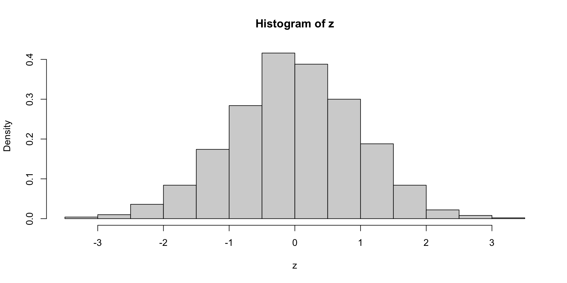
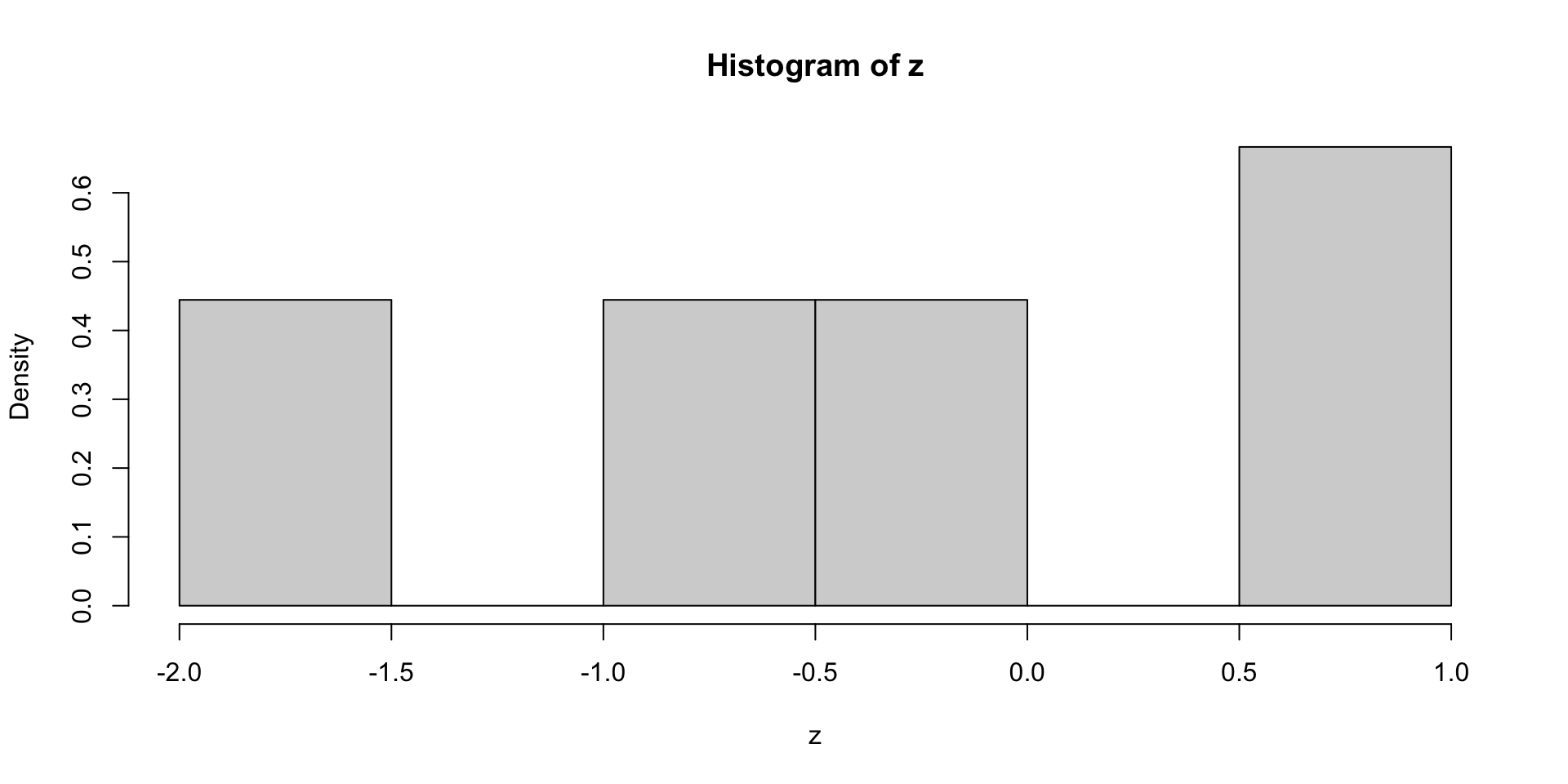
Drawback: Small samples \implies hard to check normality from histogram

• This is true even if the data is normal
• Example: z below is sample of size 9 from N(0,1) – But histogram not normal

z <- c(-0.78, -1.67, -0.38,  0.92, -0.58,  
       0.61, -1.62, -0.06, 0.52)           # Random from N(0,1)
hist(z, probability = TRUE)                # Histogram not normal

Solution: Suppose given iid sample z from a distribution f

• The command density(z) estimates the population distribution f
  (Estimate based on the sampling distribution of z and smoothing - Not easy task)

• Example: z as in previous slide. The plot of density(z) shows normal behavior

z <- c(-0.78, -1.67, -0.38,  0.92, -0.58,  
       0.61, -1.62, -0.06, 0.52)           # Random from N(0,1)
dz <- density(z)                           # Estimate the density of z
plot(dz)                                   # Plot the estimated density

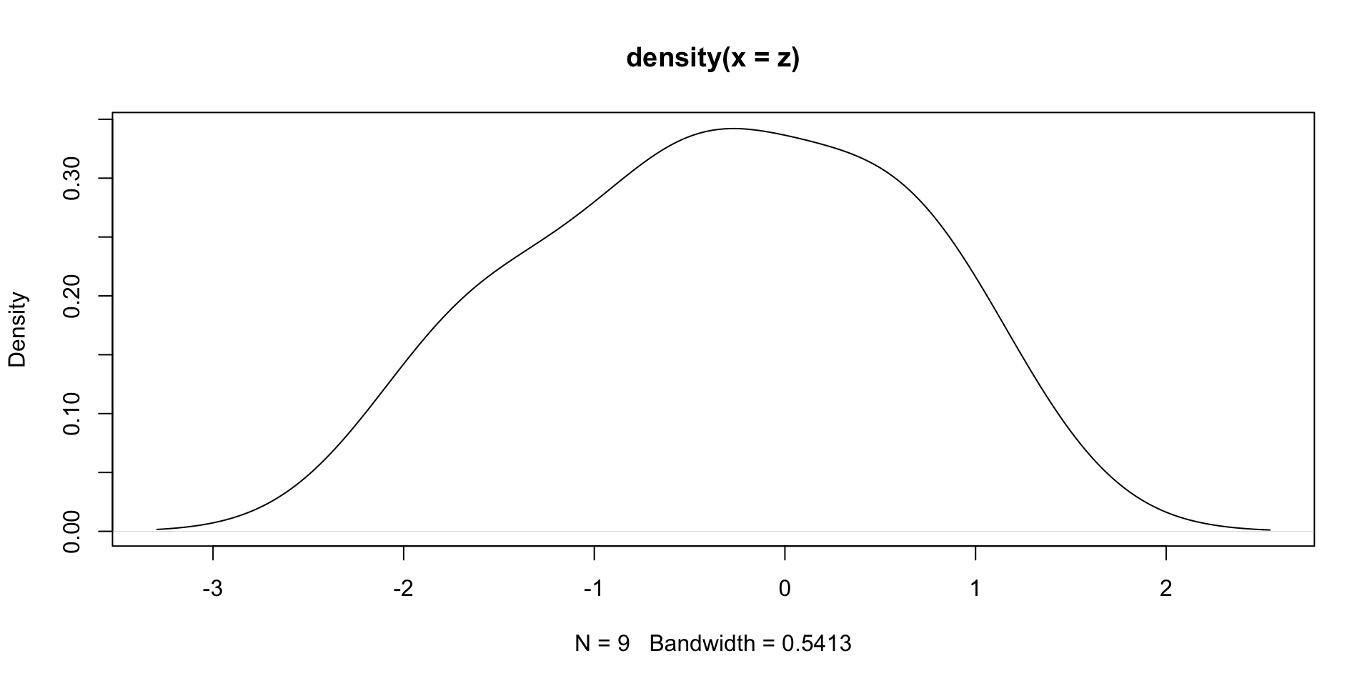
The R object density(z) models a 1D function (the estimated distribution of z)

• As such, it contains a grid of x values, with associated y values
  • x values are stored in vector density(z)$x
  • y values are stored in vector density(z)$y
• These values are useful to set the axis range in a plot

dz <- density(z)

plot(dz,                        # Plot dz
     xlim = range(dz$x),        # Set x-axis range
     ylim = range(dz$y))        # Set y-axis range

Axes range set as the min and max values of components of dz

Checking the Assumptions on our Example

# Compute the estimated distributions
d.math <- density(mathematicians)
d.acc <- density(accountants)

# Plot the estimated distributions

plot(d.math,                                    # Plot d.math
     xlim = range(c(d.math$x, d.acc$x)),        # Set x-axis range
     ylim = range(c(d.math$y, d.acc$y)),        # Set y-axis range
     main = "Estimated Distributions of Wages") # Add title to plot
lines(d.acc,                                    # Layer plot of d.acc
      lty = 2)                                  # Use different line style
         
legend("topleft",                               # Add legend at top-left
       legend = c("Mathematicians",             # Labels for legend
                  "Accountants"), 
       lty = c(1, 2))                           # Assign curves to legend

Axes range set as the min and max values of components of d.math and d.acc

1. Wages data looks approximately normally distributed (roughly bell-shaped)

2. The two populations have similar variance (spreads look similar)

Conclusion: Two-sample t-test with equal variance is appropriate \implies accept H_0

Part 7:
The Welch t-test

Samples with different variance

• We just examined the two-sample t-tests

• This assumes independent normal populations with equal variance

\sigma_X^2 = \sigma_Y^2

• Question: What happens if variances are different?

• Answer: Use the Welch Two-sample t-test

  • This is a generalization of the two-sample t-test to the case \sigma_X^2 \neq \sigma_Y^2
  • In R it is performed with t.test(x, y)
  • Note that we are just omitting the option var.equal = TRUE
  • Equivalently, you may specify var.equal = FALSE

The Welch two-sample t-test

• Welch t-test consists in computing the Welch statistic w = \frac{\overline{x} - \overline{y}}{ \sqrt{ \dfrac{s_X^2}{n} + \dfrac{s_Y^2}{m} } }

• If sample sizes m,n > 5, then w is approximately t-distributed

  • Degrees of freedom are not integer, and depend on S_X, S_Y, n, m

• If variances are similar, the welch statistic is comparable to the t-statistic

w \approx t : = \frac{ \overline{x} - \overline{y} }{s_p \sqrt{ \dfrac{1}{n} + \dfrac{1}{m} }}

Welch t-test Vs two-sample t-test

If variances are similar:

• Welch statistic and t-statistic are similar
• p-value from Welch t-test is similar to p-value from two-sample t-test
• Since p-values are similar, most times the 2 tests yield same decision
• The tests can be used interchangeably

If variances are very different:

• Welch statistic and t-statistic are different
• p-values from the two tests can differ a lot
• The two tests might give different decision
• Wrong to apply two-sample t-test, as variances are different

The Welch two-sample t-test in R

# Enter Wages data

mathematicians <- c(36, 40, 46, 54, 57, 58, 59, 60, 62, 63)
accountants <- c(37, 37, 42, 44, 46, 48, 54, 56, 59, 60, 60, 64, 64)


# Perform Welch two-sample t-test with null hypothesis mu_X = mu_Y
# Store result of t.test in answer

answer <- t.test(mathematicians, accountants)


# Print answer
print(answer)

• Note:
  • This is almost the same code as in Slide 86
  • Only difference: we are omitting the option var.equal = TRUE in t.test

    Welch Two Sample t-test

data:  mathematicians and accountants
t = 0.46546, df = 19.795, p-value = 0.6467
alternative hypothesis: true difference in means is not equal to 0
95 percent confidence interval:
 -6.566879 10.336109
sample estimates:
mean of x mean of y 
 53.50000  51.61538 

Comments on output:

1. First line: R tells us that a Welch Two-Sample t-test is performed
   • The rest of the output is similar to classic t-test
   • Main difference is that p-value and t-statistic differ from classic t-test

    Welch Two Sample t-test

data:  mathematicians and accountants
t = 0.46546, df = 19.795, p-value = 0.6467
alternative hypothesis: true difference in means is not equal to 0
95 percent confidence interval:
 -6.566879 10.336109
sample estimates:
mean of x mean of y 
 53.50000  51.61538 

Comments on output:

2. Third line:
   • The Welch t-statistic is w = 0.46546 (standard t-test gave t = 0.46359)
   • Degrees of freedom are fractionary \rm{df} = 19.795 (standard t-test \rm{df} = 21)
   • The Welch t-statistic is approximately t-distributed with W \approx t_{19.795}
3. Fifth line: The confidence interval for \mu_X - \mu_Y is also different

    Welch Two Sample t-test

data:  mathematicians and accountants
t = 0.46546, df = 19.795, p-value = 0.6467
alternative hypothesis: true difference in means is not equal to 0
95 percent confidence interval:
 -6.566879 10.336109
sample estimates:
mean of x mean of y 
 53.50000  51.61538 

Conclusion: The p-values obtained with the 2 tests are almost the same

• Welch t-test: p-value = 0.6467 \qquad Classic t-test: p-value = 0.6477

• Both test: p > 0.05, and therefore do not reject H_0

• Note: This was expected

  • The spread of the two populations is similar \implies \, \sigma_X^2 \approx \sigma_Y^2
  • Hence, Welch t-statistic approximates t-statistic \implies p-values are similar

Exercise

• We compare the Effect of Two Treatments on Blood Pressure Change

• Both treatments are given to a group of patients

• Measurements of changes in blood pressure are taken after 4 weeks of treatment

• Note that changes represent both positive and negative shifts in blood pressure

Treat. A	-1.9	-2.5	-2.1	-2.4	-2.6	-1.9
Treat. B	-1.1	-0.9	-1.4	0.2	0.3	0.6	-5	-2.4	1.5	-2.3	-2.8	2.1

# Enter changes in Blood pressure data

trA <- c(-1.9, -2.5, -2.1, -2.4, -2.6, -1.9)
trB <- c(-1.1, -0.9, -1.4, 0.2, 0.3, 0.6, -5,
         -2.4, -1.5, 2.3, -2.8, 2.1)

cat("Mean of Treatment A:", mean(trA), "Mean of Treatment B:", mean(trB))

Mean of Treatment A: -2.233333 Mean of Treatment B: -0.8

• Sample means show both Treatments are effective in decreasing blood pressure

• However Treatment A seems slightly better

Question: Perform a t-test to see if Treatment A is better H_0 \colon \mu_A = \mu_B \, , \qquad H_1 \colon \mu_A < \mu_B

Solution: Estimated density of Treatment A

plot(density(trA))    

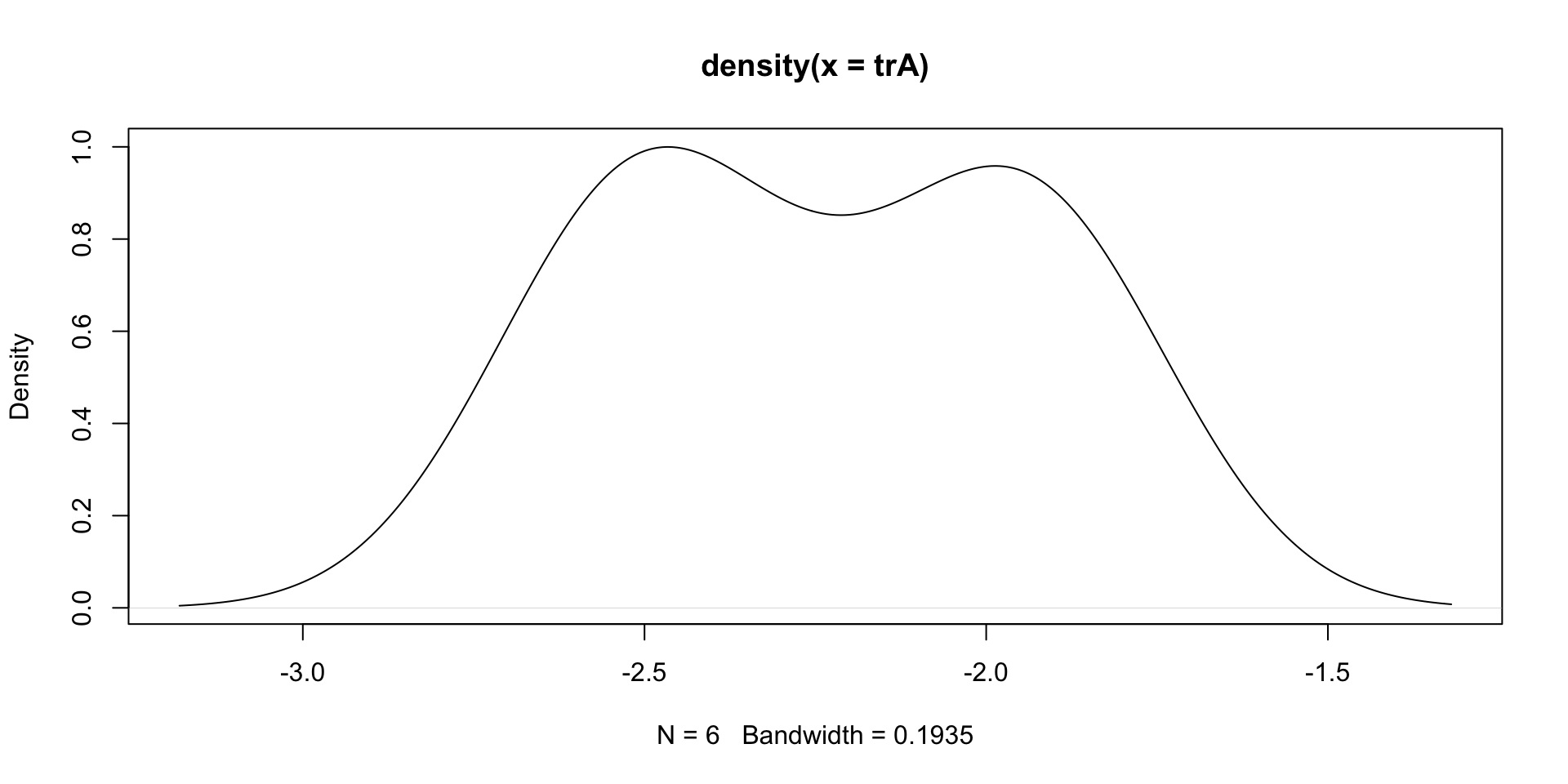
• Estimated density looks bell-shaped \implies First population is normal
• Sample seems concentrated between -3 and -1.5

Estimated density of Treatment B

plot(density(trB))    

• Estimated density looks bell-shaped \implies Second population is normal
• Sample seems concentrated between -7 and 4

Findings

• Both populations are normal \implies t-test is appropriate
• First sample seems concentrated between -3 and -1.5
• Second sample seems concentrated between -7 and 4
• Treatment B has larger spread
• Therefore we suspect that populations have different variance

\sigma_A^2 \neq \sigma_B^2

Conclusion:

• The Welch t-test is appropriate
• Two sample t-test would not be appropriate (as it assumes equal variance)

Apply the Welch t-test

We are testing the one-sided hypothesis

H_0 \colon \mu_A = \mu_B \, , \qquad H_1 \colon \mu_A < \mu_B

# Perform Welch t-test and retrieve p-value

ans <- t.test(trA, trB, alt = "less", var.equal = F) 
ans$p.value

[1] 0.01866013

• The p-value is p < 0.05

• We reject H_0 \implies Treatment A is more effective

Two-sample t-test gives different decision

We are testing the one-sided hypothesis

H_0 \colon \mu_A = \mu_B \, , \qquad H_1 \colon \mu_A < \mu_B

# Perform two-sample t-test and retrieve p-value

ans <- t.test(trA, trB, alt = "less", var.equal = T) 
ans$p.value

[1] 0.05836482

• The p-value is p > 0.05

• H_0 cannot be rejected \implies There is no evidence that Treatment A is better

• Wrong conclusion, because two-sample t-test does not apply

Disclaimer

• The previous data was synthetic, and the background story was made up!

• Nonetheless, the example is still valid

• To construct the data, I sampled as follows

  • Treatment A: Sample of size 6 from N(-2,1)
  • Treatment B: Sample of size 12 from N(-1.5,9)

• We see that \mu_A < \mu_B \,, \qquad \sigma_A^2 \neq \sigma_B^2

• This tells us that:

  • We can expect that some samples will support that \mu_A < \mu_B
  • Two-sample t-test is inappropriate because \sigma_A^2 \neq \sigma_B^2

Generating the Data

# Set seed for random generation
# This way you always get the same random numbers when
# you run this code
set.seed(21) 

repeat {
  # Generate random samples
  x <- rnorm(6, mean = -2, sd = 1)
  y <- rnorm(12, mean = -1.5, sd = 3)

  # Round x and y to 1 decimal point
  x <- round(x, 1)
  y <- round(y, 1)
  
  # Perform one-sided t-tests for alternative hypothesis mu_x < mu_y 
  ans_welch <- t.test(x, y, alt = "less", var.equal = F)
  ans_t_test <- t.test(x, y, alt = "less", var.equal = T)
   
  # Check that Welch test succeeds and two-sample test fails
  if (ans_welch$p.value < 0.05 && ans_t_test$p.value > 0.05) {
    cat("Data successfully generated!!!\n\n")
    cat("Synthetic Data TrA:", x, "\n")
    cat("Synthetic Data TrB:", y, "\n\n")
    cat("Welch t-test p-value:", ans_welch$p.value, "\n")
    cat("Two-sample t-test p-value:", ans_t_test$p.value)
    break
    }
}

Data successfully generated!!!

Synthetic Data TrA: -1.9 -2.5 -2.1 -2.4 -2.6 -1.9 
Synthetic Data TrB: -1.1 -0.9 -1.4 0.2 0.3 0.6 -5 -2.4 -1.5 2.3 -2.8 2.1 

Welch t-test p-value: 0.01866013 
Two-sample t-test p-value: 0.05836482

Method:

• Sample the data as in previous slide (round to 1 d.p. for cleaner looking data)

• Repeat until Welch test succeeds, and two-sample t-test fails \text{p-value of Welch test } \, < 0.05 < \, \text{p-value of Two-sample t-test}

Part 8:
The t-test for
paired samples

Paired samples

• Assume to have two sample with same size

• Sometimes the two samples depend on each other in some way

1. Twin studies:
   • Twins are used as pairs (to control genetic or environmental factors)
   • Example: test effectiveness of a medical treatment against placebo
   • The two samples are clearly dependent
     (think of twins as the same person)
     
   • As such, the usual two-sample t-test is not applicable
     (because it assumes independence)

Paired samples

• Assume to have two sample with same size

• Sometimes the two samples depend on each other in some way

2. Pre-test and Post-test
   • Measure the outcome of a certain action
   • Example: does this module work for teaching R?
   • We can assess the effectiveness of something with a pre-test and a post-test
   • The two samples are clearly dependent
     (each individual takes a test twice)
   • As such, the usual two-sample t-test is not applicable
     (because it assumes independence)

The paired t-test

Suppose given two samples

• Sample x_1, \ldots, x_n from N(\mu_X,\sigma^2_X)

• Sample y_1, \ldots, y_n from N(\mu_Y,\sigma^2_Y)

The hypotheses for difference in means are H_0 \colon \mu_X = \mu_Y \,, \quad \qquad H_1 \colon \mu_X \neq \mu_Y \,, \quad \mu_X < \mu_Y \,, \quad \text{ or } \quad \mu_X > \mu_Y

The paired t-test

Assumption: The data is paired, meaning that the differences

d_i = x_i - y_i \,\, \text{ are iid} \,\, N(\mu,\sigma^2) \quad \text{where} \quad \mu := \mu_X - \mu_Y

The hypotheses for the difference in means are equivalent to

H_0 \colon \mu = 0 \,, \quad \qquad H_1 \colon \mu \neq 0 \,, \quad \mu < 0 \,, \quad \text{ or } \quad \mu > 0

These can be tested with a one-sample t-test

R commands: The paired t-test can be called with the equivalent commands

• t.test(x, y, paired = TRUE) \qquad \quad H_0 \colon \mu_X = \mu_Y

• t.test(x - y) \qquad \qquad \qquad \qquad\qquad H_0 \colon \mu = 0

Example 1: The 2008 crisis (again!)

Month	J	F	M	A	M	J	J	A	S	O	N	D
CCI 2007	86	86	88	90	99	97	97	96	99	97	90	90
CCI 2009	24	22	21	21	19	18	17	18	21	23	22	21

• Data: Monthly Consumer Confidence Index (CCI) in 2007 and 2009

• Question: Did the crash of 2008 have lasting impact upon CCI?

• Observations:

  • Data shows a massive drop in CCI between 2007 and 2009
  • Data is clearly paired (Pre-test and Post-test situation)

• Method: Use paired t-test to investigate drop in mean CCI

H_0 \colon \mu_{2007} = \mu_{2009} \,, \quad H_1 \colon \mu_{2007} > \mu_{2009}

Perform paired t-test

# Enter CCI data
score_2007 <- c(86, 86, 88, 90, 99, 97, 97, 96, 99, 97, 90, 90)
score_2009 <- c(24, 22, 21, 21, 19, 18, 17, 18, 21, 23, 22, 21)

# Perform paired t-test and print p-value
ans <- t.test(score_2007, score_2009, paired = T, alt = "greater")
ans$p.value

[1] 2.430343e-13

The p-value is significant: \,\, p < 0.05 \, \implies \, reject H_0 \, \implies \, Drop in CCI

Warning

It would be wrong to use a two-sample t-test

• This is because the samples are paired, and hence dependent

• This is further supported by computing the correlation

• High correlation implies dependence

cor(score_2007, score_2009)                # Correlation is high

[1] -0.6076749

Example 2: Water quality samples

• Researchers wish to measure water quality

• There are two possible tests, one less expensive than the other

• 10 water samples were taken, and each was measured both ways

method1	45.9	57.6	54.9	38.7	35.7	39.2	45.9	43.2	45.4	54.8
method2	48.2	64.2	56.8	47.2	43.7	45.7	53.0	52.0	45.1	57.5

Question: Do the tests give the same results?

• Observation: The data is paired (twin study situation)

• Method: Use paired t-test to investigate equality of results

H_0 \colon \mu_1 = \mu_2 \,, \quad H_1 \colon \mu_1 \neq \mu_2

Perform paired t-test

# Enter tests data
method1 <- c(45.9, 57.6, 54.9, 38.7, 35.7, 39.2, 45.9, 43.2, 45.4, 54.8)
method2 <- c(48.2, 64.2, 56.8, 47.2, 43.7, 45.7, 53.0, 52.0, 45.1, 57.5)

# Perform paired t-test and print p-value
ans <- t.test(method1, method2, paired = T)
ans$p.value

[1] 0.0006648526

p-value is significant: \,\, p < 0.05 \implies reject H_0 \implies Methods perform differently

Warning

It would be wrong to use a two-sample t-test

• This is because the samples are paired, and hence dependent

• This is also supported by high samples correlation

cor(method1, method2)                # Correlation is very high

[1] 0.9015147

Warning

In this Example, performing a two-sample t-test would lead to wrong decision

# Perform Welch t-test and print p-value
ans <- t.test(method1, method2, paired = F)       # paired = F is default
ans$p.val

[1] 0.1165538

Wrong conclusion: \,\, p > 0.05 \implies can’t reject H_0 \implies Methods perform similarly

Bottom line: The data is paired, therefore a paired t-test must be used

Part 1:
The F-distribution

Recall

The chi-squared distribution with p degrees of freedom is \chi_p^2 = Z_1^2 + \ldots + Z_p^2 \qquad \text{where} \qquad Z_1, \ldots, Z_n \,\,\, \text{iid} \,\,\, N(0, 1)

Chi-squared distribution was used to:

• Describe distribution of sample variance S^2: \frac{(n-1)S^2}{\sigma^2} \sim \chi_{n-1}^2

• Define t-distribution with p degrees of freedom: t_p \sim \frac{U}{\sqrt{V/p}} \qquad \text{where} \qquad U \sim N(0,1) \,, \quad V \sim \chi_p^2 \quad \text{ independent}

The F-distribution

Definition

The r.v. F has F-distribution with p and q degrees of freedom if the pdf is f_F(x) = \frac{ \Gamma \left(\frac{p+q}{2} \right) }{ \Gamma \left( \frac{p}{2} \right) \Gamma \left( \frac{q}{2} \right) } \left( \frac{p}{q} \right)^{p/2} \, \frac{ x^{ (p/2) - 1 } }{ [ 1 + (p/q) x ]^{(p+q)/2} } \,, \quad x > 0

Notation: F-distribution with p and q degrees of freedom is denoted by F_{p,q}

Remark: Used to describes variance estimators for independent samples

Plot of F-distributions

Characterization of F-distribution

The F-distribution is obtained as ratio of 2 independent chi-squared distributions

Theorem

Suppose that U \sim \chi_p^2 and V \sim \chi_q^2 are independent. Then X := \frac{U/p}{V/q} \sim F_{p,q}

Idea of Proof

• This is similar to the proof (seen in Homework 2) that \frac{U}{\sqrt{V/p}} \sim t_p where U \sim N(0,1) and V \sim \chi_p^2 are independent

• In our case we need to prove X := \frac{U/p}{V/q} \sim F_{p,q} where U \sim \chi_p^2 and V \sim \chi_q^2 are independent

Idea of Proof

• U \sim \chi_{p}^2 and V \sim \chi_q^2 are independent. Therefore \begin{align*} f_{U,V} (u,v) & = f_U(u) f_V(v) \\ & = \frac{ 1 }{ \Gamma \left( \frac{p}{2} \right) \Gamma \left( \frac{q}{2} \right) 2^{(p+q)/2} } u^{\frac{p}{2} - 1} v^{\frac{q}{2} - 1} e^{-(u+v)/2} \end{align*}

• Consider the change of variables x(u,v) := \frac{u/p}{v/q} \,, \quad y(u,v) := u + v

Idea of Proof

• This way we have X = \frac{U/p}{V/q} \,, \qquad Y = U + V

• To conclude the proof, we need to compute the pdf of X, that is f_X

• This can be computed as the X marginal of f_{X,Y} f_{X}(x) = \int_{0}^\infty f_{X,Y}(x,y) \, dy

Idea of Proof

• The joint pdf f_{X,Y} can be computed by inverting the change of variables x(u,v) := \frac{u/p}{v/q} \,, \quad y(u,v) := u + v and using the formula f_{X,Y}(x,y) = f_{U,V}(u(x,y),v(x,y)) \, |\det J| where J is the Jacobian of the inverse transformation (x,y) \mapsto (u(x,y),v(x,y))

Idea of Proof

• Since f_{U,V} is known, then also f_{X,Y} is known

• Moreover the integral f_{X}(x) = \int_{0}^\infty f_{X,Y}(x,y) \, dy can be explicitly computed, yielding the thesis f_{X}(x) = \frac{ \Gamma \left(\frac{p+q}{2} \right) }{ \Gamma \left( \frac{p}{2} \right) \Gamma \left( \frac{q}{2} \right) } \left( \frac{p}{q} \right)^{p/2} \, \frac{ x^{ (p/2) - 1 } }{ [ 1 + (p/q) x ]^{(p+q)/2} }

Properties of F-distribution

Theorem

1. Suppose X \sim F_{p,q} with q>2. Then {\rm I\kern-.3em E}[X] = \frac{q}{q-2}

2. If X \sim F_{p,q} then 1/X \sim F_{q,p}

3. If X \sim t_q then X^2 \sim F_{1,q}

Properties of F-distribution

Proof of Theorem

1. Requires a bit of work (omitted)

2. By the Theorem in Slide 6, we have X \sim F_{p,q} \quad \implies \quad X = \frac{U/p}{V/q} with U \sim \chi_p^2 and V \sim \chi_q^2 independent. Therefore \frac{1}{X} = \frac{V/q}{U/p} \sim \frac{\chi^2_q/q}{\chi^2_p/p} \sim F_{q,p}

Properties of F-distribution

Proof of Theorem

3. Suppose X \sim t_q. The Theorem in Slide 118 of Lecture 2, guarantees that X = \frac{U}{\sqrt{V/q}} where U \sim N(0,1) and V \sim \chi_q^2 are independent. Therefore X^2 = \frac{U^2}{V/q}

Properties of F-distribution

Proof of Theorem

• Since U \sim N(0,1), by definition U^2 \sim \chi_1^2.
• Moreover U^2 and V are independet, since U and V are independent
• Finally, the Theorem in Slide 6 implies X^2 = \frac{U^2}{V/q} \sim \frac{\chi_1^2/1}{\chi_q^2/q} \sim F_{1,q}

Part 2:
Two-sample F-test

Variance estimators

Suppose given independent random samples from 2 normal populations:

• X_1, \ldots, X_n iid random sample from N(\mu_X, \sigma_X^2)
• Y_1, \ldots, Y_m iid random sample from N(\mu_Y, \sigma_Y^2)

Problem:

• We want to compare variance of the 2 populations
• We do it by studying the variances ratio \frac{\sigma_X^2}{\sigma_Y^2}

Variance estimators

Question:

• Suppose the variances \sigma_X^2 and \sigma_Y^2 are unknown
• How can we estimate the ratio \sigma_X^2 /\sigma_Y^2 \, ?

Answer:

• Estimate the ratio \sigma_X^2 /\sigma_Y^2 \, using sample variances S^2_X / S^2_Y

• The F-distribution allows to compare the quantities \sigma_X^2 /\sigma_Y^2 \qquad \text{and} \qquad S^2_X / S^2_Y

Variance ratio distribution

Theorem

Suppose given independent random samples from 2 normal populations:

• X_1, \ldots, X_n iid random sample from N(\mu_X, \sigma_X^2)
• Y_1, \ldots, Y_m iid random sample from N(\mu_Y, \sigma_Y^2)

The random variable F = \frac{ S_X^2 / \sigma_X^2 }{ S_Y^2 / \sigma_Y^2 } \, \sim \, F_{n-1,m-1} that is, F is F-distributed with n-1 and m-1 degrees of freedom

Variance ratio distribution

Proof

• We need to prove F = \frac{ S_X^2 / \sigma_X^2 }{ S_Y^2 / \sigma_Y^2 } \sim F_{n-1,m-1}

• By the Theorem in Slide 101 Lecture 2, we have that \frac{S_X^2}{ \sigma_X^2} \sim \frac{\chi_{n-1}^2}{n-1} \,, \qquad \frac{S_Y^2}{ \sigma_Y^2} \sim \frac{\chi_{m-1}^2}{m-1}

Variance ratio distribution

Proof

• Therefore F = \frac{ S_X^2 / \sigma_X^2 }{ S_Y^2 / \sigma_Y^2 } = \frac{U/p}{V/q} where we have U \sim \chi_{p}^2 \,, \qquad V \sim \chi_q^2 \,, \qquad p = n-1 \,, \qquad q = m - 1

• By the Theorem in Slide 6, we infer the thesis F = \frac{U/p}{V/q} \sim F_{n-1,m-1}

Unbiased estimation of variance ratio

Question: Why is S_X^2/S_Y^2 a good estimator for \sigma_X^2/\sigma_Y^2

Answer:

• Because S_X^2/S_Y^2 is (asymptotically) unbiased estimator of \sigma_X^2/\sigma_Y^2
• This is shown in the following Theorem

Unbiased estimation of variance ratio

Theorem

Suppose given independent random samples from 2 normal populations:

• X_1, \ldots, X_n iid random sample from N(\mu_X, \sigma_X^2)
• Y_1, \ldots, Y_m iid random sample from N(\mu_Y, \sigma_Y^2)

It holds that {\rm I\kern-.3em E}\left[ \frac{S_X^2}{S_Y^2} \right] = \frac{m-1}{m-3} \frac{\sigma_X^2}{\sigma_Y^2} \,, \qquad \lim_{m \to \infty} {\rm I\kern-.3em E}\left[ \frac{S_X^2}{S_Y^2} \right] = \frac{\sigma_X^2}{\sigma_Y^2}

The F-statistic

Assumption: Suppose given 2 samples from independent normal populations

X_1, \ldots, X_n \, \text{ iid from } \, N(\mu_X, \sigma_X^2) \,, \qquad \quad Y_1, \ldots, Y_m \, \text{ iid from } \, N(\mu_Y, \sigma_Y^2)

Definition

The F-statistic is defined as F := \frac{ S_X^2 / \sigma_X^2 }{ S_Y^2 / \sigma_Y^2 } \, \sim \, F_{n-1,m-1}

Note: Under the Null hypothesis that \sigma_X^2 = \sigma_Y^2, the F-statistic simplifies to F = \frac{ S_X^2 }{ S_Y^2 }

The two-sample F-test

Suppose given two independent samples

x_1, \ldots, x_n \, \text{ iid from } \, N(\mu_X, \sigma_X^2) \,, \qquad \quad y_1, \ldots, y_m \, \text{ iid from } \, N(\mu_Y, \sigma_Y^2)

The hypotheses for difference in variance are H_0 \colon \sigma_X^2 = \sigma_Y^2 \,, \quad \qquad H_1 \colon \sigma_X^2 \neq \sigma_Y^2 \quad \text{ or } \quad H_1 \colon \sigma_X^2 > \sigma_Y^2

Very important: We only consider two-sided and right-tailed hypotheses

• This is because we can always label the samples in a way that s_X^2 \geq s_Y^2

• Therefore, there is no reason to suspect that \sigma_X^2 < \sigma_Y^2

• This allows us to work only with upper quantiles
  (and avoid a lot of trouble, as the F-distribution is asymmetric)

Procedure: 3 Steps

1. Calculation: Compute the two-sample F-statistic F = \frac{ s_X^2}{ s_Y^2} where sample variances are s_X^2 = \frac{\sum_{i=1}^n x_i^2 - n \overline{x}^2}{n-1} \qquad \quad s_Y^2 = \frac{\sum_{i=1}^m y_i^2 - m \overline{y}^2}{m-1}

Very important: s_X^2 refers to the sample with largest variance

\implies \quad s_X^2 \geq s_Y^2 \,, \qquad F \geq 1

2. Statistical Tables or R: Find either
   • Critical value F^* in Tables 3, 4
   • p-value in R

3. Interpretation: Reject H_0 when either p < 0.05 \qquad \text{ or } \qquad F \in \,\,\text{Rejection Region} \qquad \qquad \qquad \qquad (X \, \sim \, F_{n-1,m-1})

Alternative	Rejection Region	F^*	p-value
\sigma^2_X \neq \sigma^2_Y	F > F^*	F_{n-1, m-1}(0.025)	2P(X > F)
\sigma^2_X > \sigma^2_Y	F > F^*	F_{n -1, m-1}(0.05)	P(X > F)

• Reject H_0 if F-statistic falls in the Rejection Region (in gray)

• Recall F \geq 1 \implies for two-sided test we only need to check if F > F_{n-1,m-1}(0.025)

Tables: Critical values of F distribution

• Always construct F-statistic as F = \frac{s^2_X}{s^2_Y} \quad\quad \text{where} \quad\quad s^2_X \geq s^2_Y \qquad \implies \qquad F \geq 1

• This way only the upper critical values of F-distribution are needed

• Upper critical values for F distribution are in Tables 3, 4

Table #	Critical values
3	F_{\nu_1,\nu_2} (0.05)
4	F_{\nu_1,\nu_2} (0.025)

Table 3 in Statistics_Tables.pdf

Table 3: Lists the values F_{\nu_1,\nu_2}(0.05), which means

P(X > F_{\nu_1,\nu_2}(0.05)) = 0.05 \,, \qquad \text{ when } \quad X \sim F_{\nu_1,\nu_2}

For example F_{9, 6}(0.05) = 4.10

Plot of F_{9,6} distribution. White area is 0.95. Shaded area is 0.05 P(F_{9,6} > 4.10) = 0.05 \,, \qquad 4.10 = F_{9,6}(0.05)

Table 4 in Statistics_Tables.pdf

Table 4: Lists the values F_{\nu_1,\nu_2}(0.025), which means

P(X > F_{\nu_1,\nu_2}(0.025)) = 0.025 \,, \qquad \text{ when } \quad X \sim F_{\nu_1,\nu_2}

For example F_{9, 6}(0.025) = 5.52

What about missing values?

• Sometimes the value F_{\nu_1,\nu_2}(\alpha) is missing from F-table

• In such case approximate F_{\nu_1,\nu_2}(\alpha) with average of closest entries available

Example: F_{21,5}(0.05) is missing. We can approximate it by F_{21,5}(0.05) \approx \frac{F_{20,5}(0.05) + F_{25,5}(0.05)}{2} = \frac{ 4.56 + 4.52 }{ 2 } = 4.54

The two-sample F-test in R

1. Store the samples x_1,\ldots,x_n and y_1,\ldots,y_m in two R vectors
   • x <- c(x1, ..., xn)
   • y <- c(y1, ..., ym)
2. Perform a two-sample F-test on x and y

Alternative	R command
\sigma_X^2 \neq \sigma_Y^2	var.test(x, y)
\sigma_X^2 > \sigma_Y^2	var.test(x, y, alt = "greater")

3. Read output: similar to two-sample t-test
   • The main quantity of interest is p-value

Part 3:
Worked Example

• Data: Wages of 10 Mathematicians and 13 Accountants (again!)

• Assumptions: Wages are independent and normally distributed

Mathematicians	36	40	46	54	57	58	59	60	62	63
Accountants	37	37	42	44	46	48	54	56	59	60	60	64	64

• Last week, we conducted a two-sample t-test for equality of means H_0 \colon \mu_X = \mu_Y \,, \qquad H_1 \colon \mu_X \neq \mu_Y

• We concluded that there is no evidence (p>0.05) of difference in pay levels

• However, the two-sample t-test assumed equal variance \sigma_X^2 = \sigma_Y^2

• We checked this assumption by plotting the estimated sample distributions

# Enter the Wages data
mathematicians <- c(36, 40, 46, 54, 57, 58, 59, 60, 62, 63)
accountants <- c(37, 37, 42, 44, 46, 48, 54, 56, 59, 60, 60, 64, 64)

# Compute the estimated distributions
d.math <- density(mathematicians)
d.acc <- density(accountants)

# Plot the estimated distributions

plot(d.math,                                    # Plot d.math
     xlim = range(c(d.math$x, d.acc$x)),        # Set x-axis range
     ylim = range(c(d.math$y, d.acc$y)),        # Set y-axis range
     main = "Estimated Distributions of Wages") # Add title to plot
lines(d.acc,                                    # Layer plot of d.acc
      lty = 2)                                  # Use different line style
         
legend("topleft",                               # Add legend at top-left
       legend = c("Mathematicians",             # Labels for legend
                  "Accountants"), 
       lty = c(1, 2))                           # Assign curves to legend          

• The plot shows that the two populations have similar variance (spread)

• Thanks to the F-test, we can now compare variances in a quantitative way

Setting up the F-test

• We want to test for equality of the two variances

• There is no prior reason to believe that pay in one group is more spread out

• Therefore, a two-sided test is appropriate H_0 \colon \sigma_X^2 = \sigma_Y^2 \,, \qquad H_1 \colon \sigma_X^2 \neq \sigma_Y^2

• First task is to compute the F-statistic F = \frac{s_X^2}{s_Y^2}

• Important: We need to make sure the samples are labelled so that s_X^2 \geq s_Y^2

1. Calculation

Variance of first sample (Already done last week!)

• Sample size: \ n = No. of Mathematicians = 10

• Mean: \bar{x} = \frac{\sum_{i=1}^n x_i}{n} = \frac{36+40+46+ \ldots +62+63}{10}=\frac{535}{10}=53.5

• Variance: \begin{align*} \sum_{i=1}^n x_i^2 & = 36^2+40^2+46^2+ \ldots +62^2+63^2 = 29435 \\ s^2_X & = \frac{\sum_{i=1}^n x_i^2 - n \bar{x}^2}{n -1 } = \frac{29435-10(53.5)^2}{9} = 90.2778 \end{align*}

1. Calculation

Variance of second sample (Already done last week!)

• Sample size: \ m = No. of Accountants = 13

• Mean: \bar{y} = \frac{37+37+42+ \dots +64+64}{13} = \frac{671}{13} = 51.6154

• Variance: \begin{align*} \sum_{i=1}^m y_i^2 & = 37^2+37^2+42^2+ \ldots +64^2+64^2 = 35783 \\ s^2_Y & = \frac{\sum_{i=1}^m y_i^2 - m \bar{y}^2}{m - 1} = \frac{35783-13(51.6154)^2}{12} = 95.7547 \end{align*}

1. Calculation

The F-statistic

• Notice that s^2_Y = 95.7547 > 90.2778 = s_X^2

• Hence the F-statistic is F = \frac{s^2_Y}{s_X^2} = \frac{95.7547}{90.2778} = 1.061\ \quad (3\ \text{d.p.})

• Important: We have swapped role of s^2_X and s^2_Y, since s^2_Y > s^2_X. This way F > 1

2. Referencing Tables

• Degrees of freedom are n - 1 = 10 - 1 = 9 \,, \qquad m - 1 = 13 - 1 = 12

• Note: Since we have swapped role of s^2_X and s^2_Y, we have F = \frac{s^2_Y}{s_X^2} \sim F_{m-1,n-1} = F_{12,9}

• We need to find the critical value F_{12,9}(0.025) in Table 4

Note: This is a two-sided test. Hence \alpha = 0.025, and not 0.05!

• Below is a section of Table 4

• We note that F_{12, 9} is missing. Closest values are F_{10, 9} and F_{15, 9}

• We estimate the desired critical value by averaging the two

F_{12, 9}(0.025) \approx \frac{F_{10, 9}(0.025) + F_{15, 9}(0.025)}{2} = \frac{3.96 + 3.77}{2} = 3.865

3. Interpretation

• We have that F = 1.061 < 3.865 = F_{12, 9}(0.025)

• Therefore the p-value satisfies p > 0.05

• There is no evidence (p > 0.05) in favor of H_1. We have no reason to doubt that \sigma_X^2 = \sigma_Y^2

• Conclusion:

  1. Wage levels for the two groups appear to be equally well spread out
  2. This is in line with previous graphical checks

The F-test in R

We present two implementations in R:

1. Simple solution using the command var.test
2. A first-principles construction closer to our earlier hand calculation

Simple solution: var.test

This is a two-sided F-test. The p-value is computed by

p = 2 P(F_{m-1, n-1} > F) \,, \qquad F = \frac{s_Y^2}{s_X^2}

# Enter Wages data in 2 vectors using function c()
mathematicians <- c(36, 40, 46, 54, 57, 58, 59, 60, 62, 63)
accountants <- c(37, 37, 42, 44, 46, 48, 54, 56, 59, 60, 60, 64, 64)


# Perform two-sided F-test using var.test
# Store result and print
ans <- var.test(accountants, mathematicians)
print(ans)

• Note: accountants goes first because it has larger variance
• Code can be downloaded here F_test.R

    F test to compare two variances

data:  accountants and mathematicians
F = 1.0607, num df = 12, denom df = 9, p-value = 0.9505
alternative hypothesis: true ratio of variances is not equal to 1
95 percent confidence interval:
 0.2742053 3.6443547
sample estimates:
ratio of variances 
          1.060686 

Comments:

1. First line: R tells us that an F-test is performed

2. Second line: Data for F-test is accountants and mathematicians

3. The F-statistic computed is F = 1.0607

   • Note: This coincides with the one computed by hand (up to rounding error)

    F test to compare two variances

data:  accountants and mathematicians
F = 1.0607, num df = 12, denom df = 9, p-value = 0.9505
alternative hypothesis: true ratio of variances is not equal to 1
95 percent confidence interval:
 0.2742053 3.6443547
sample estimates:
ratio of variances 
          1.060686 

Comments:

4. Numerator of F-statistic has 12 degrees of freedom
5. Denominator of F-statistic has 9 degrees of freedom
6. p-value is p = 0.9505

    F test to compare two variances

data:  accountants and mathematicians
F = 1.0607, num df = 12, denom df = 9, p-value = 0.9505
alternative hypothesis: true ratio of variances is not equal to 1
95 percent confidence interval:
 0.2742053 3.6443547
sample estimates:
ratio of variances 
          1.060686 

Comments:

7. Fourth line: The alternative hypothesis is that ratio of variances is \, \neq 1
   • This translates to H_1 \colon \sigma_Y^2 \neq \sigma^2_X
   • Warning: This is not saying to reject H_0 – R is just stating H_1

    F test to compare two variances

data:  accountants and mathematicians
F = 1.0607, num df = 12, denom df = 9, p-value = 0.9505
alternative hypothesis: true ratio of variances is not equal to 1
95 percent confidence interval:
 0.2742053 3.6443547
sample estimates:
ratio of variances 
          1.060686 

Comments:

8. Fifth line: R computes a 95 \% confidence interval for ratio \sigma_Y^2/\sigma_X^2 (\sigma_Y^2/\sigma_X^2 ) \in [0.2742053, 3.6443547]
   • Interpretation: If you repeat the experiment (on new data) over and over, the interval will contain \sigma_Y^2/\sigma_X^2 about 95\% of the times

    F test to compare two variances

data:  accountants and mathematicians
F = 1.0607, num df = 12, denom df = 9, p-value = 0.9505
alternative hypothesis: true ratio of variances is not equal to 1
95 percent confidence interval:
 0.2742053 3.6443547
sample estimates:
ratio of variances 
          1.060686 

Comments:

9. Seventh line: R computes ratio of sample variances
   • We have that s_Y^2/s_X^2 = 1.060686
   • By definition, the above coincides with the F-statistic (up to rounding)

    F test to compare two variances

data:  accountants and mathematicians
F = 1.0607, num df = 12, denom df = 9, p-value = 0.9505
alternative hypothesis: true ratio of variances is not equal to 1
95 percent confidence interval:
 0.2742053 3.6443547
sample estimates:
ratio of variances 
          1.060686 

Conclusion: The p-value is p = 0.9505

• Since p > 0.05, we do not reject H_0
• Hence \sigma^2_X and \sigma^2_Y appear to be similar
• Wage levels for the two groups appear to be equally well spread out

First principles solution

• Start by entering data into R

# Enter Wages data in 2 vectors using function c()

mathematicians <- c(36, 40, 46, 54, 57, 58, 59, 60, 62, 63)
accountants <- c(37, 37, 42, 44, 46, 48, 54, 56, 59, 60, 60, 64, 64)

First principles solution

• Check which population has higher variance
• In our case accountants has higher variance

# Check which variance is higher

cat("\n Variance of accountants is", var(accountants))
cat("\n Variance of mathematicians is", var(mathematicians))

 Variance of accountants is 95.75641

 Variance of mathematicians is 90.27778

First principles solution

• Compute sample sizes

# Calculate sample sizes

n <- length(mathematicians)
m <- length(accountants)

First principles solution

• Compute F-statistic F = \frac{s_Y^2}{s_X^2}

• Recall: Numerator has to have larger variance

• In our case accountants is numerator

# Compute F-statistics
# Numerator is population with largest variance

F <- var(accountants) / var(mathematicians)

First principles solution

• Compute the p-value p = 2P(F_{m-1, n-1} > F) = 2 - 2P(F_{m-1, n-1} \leq F) \,, \qquad F = \frac{s_Y^2}{s_X^2}

# Compute p-value
p_value <- 2 - 2 * pf(F, df1 = m - 1, df2 = n - 1)

# Print p-value
cat("\n The p-value for two-sided F-test is", p_value)

• Note: The command pf(x, df1 = n, df2 = m) computes probability P(F_{n,m} \leq x)

First principles solution: Output

• Full code be downloaded here F_test_first_principles.R

• Running the code yields the output:

 Variance of accountants is 95.75641

 Variance of mathematicians is 90.27778

 The p-value for two-sided F-test is 0.9505368

• Note: The p-value coincides with the one obtained with var.test
  • This is a way to cross check our code is right
• Since p > 0.05, we do not reject H_0