Statistical Models

Lecture 2

Dr. Silvio Fanzon

S.Fanzon@hull.ac.uk

University of Hull

Lecture 2:
Random samples &
The t-test

Outline of Lecture 2

1. Multivariate random vectors
2. Random samples
3. Unbiased estimators
4. Chi-squared distribution
5. Sampling from normal distribution
6. t-distribution
7. Hypothesis testing
8. The one-sample t-test

Part 1:
Multivariate random vectors

Multivariate Random Vectors

Recall

• A Random vector is a function \mathbf{X}\colon \Omega \to \mathbb{R}^n
• \mathbf{X} is a multivariate random vector if n \geq 3
• We denote the components of \mathbf{X} by \mathbf{X}= (X_1,\ldots,X_n) \,, \qquad X_i \colon \Omega \to \mathbb{R}
• We denote the components of a point \mathbf{x}\in \mathbb{R}^n by \mathbf{x}= (x_1,\ldots,x_n)

Discrete and Continuous Multivariate Random Vectors

Everything we defined for bivariate vectors extends to multivariate vectors

Definition

The random vector \mathbf{X}\colon \Omega \to \mathbb{R}^n is:

• continuous if components X_is are continuous
• discrete if components X_i are discrete

Joint pmf

Definition

The joint pmf of a continuous random vector \mathbf{X} is f_{\mathbf{X}} \colon \mathbb{R}^n \to \mathbb{R} defined by f_{\mathbf{X}} (\mathbf{x}) = f_{\mathbf{X}}(x_1,\ldots,x_n) := P(X_1 = x_1 , \ldots , X_n = x_n ) \,, \qquad \forall \, \mathbf{x}\in \mathbb{R}^n

Note: For all A \subset \mathbb{R}^n it holds P(\mathbf{X}\in A) = \sum_{\mathbf{x}\in A} f_{\mathbf{X}}(\mathbf{x})

Joint pdf

Definition

The joint pdf of a continuous random vector \mathbf{X} is a function f_{\mathbf{X}} \colon \mathbb{R}^n \to \mathbb{R} such that P (\mathbf{X}\in A) := \int_A f_{\mathbf{X}}(x_1 ,\ldots, x_n) \, dx_1 \ldots dx_n = \int_{A} f_{\mathbf{X}}(\mathbf{x}) \, d\mathbf{x}\,, \quad \forall \, A \subset \mathbb{R}^n

Note: \int_A denotes an n-fold intergral over all points \mathbf{x}\in A

Expected Value

Definition

\mathbf{X}\colon \Omega \to \mathbb{R}^n random vector and g \colon \mathbb{R}^n \to \mathbb{R} function. The expected value of the random variable g(X) is \begin{align*} {\rm I\kern-.3em E}[g(\mathbf{X})] & := \sum_{x \in \mathbb{R}^n} g(\mathbf{x}) f_{\mathbf{X}} (\mathbf{x}) \qquad & (\mathbf{X}\text{ discrete}) \\ {\rm I\kern-.3em E}[g(\mathbf{X})] & := \int_{\mathbb{R}^n} g(\mathbf{x}) f_{\mathbf{X}} (\mathbf{x}) \, d\mathbf{x}\qquad & \qquad (\mathbf{X}\text{ continuous}) \end{align*}

Marginal distributions

• Marginal pmf or pdf of any subset of the coordinates (X_1,\ldots,X_n) can be computed by integrating or summing the remaining coordinates

• To ease notations, we only define maginals wrt the first k coordinates

Definition

The marginal pmf or marginal pdf of the random vector \mathbf{X} with respect to the first k coordinates is the function f \colon \mathbb{R}^k \to \mathbb{R} defined by \begin{align*} f(x_1,\ldots,x_k) & := \sum_{ (x_{k+1}, \ldots, x_n) \in \mathbb{R}^{n-k} } f_{\mathbf{X}} (x_1 , \ldots , x_n) \quad & (\mathbf{X}\text{ discrete}) \\ f(x_1,\ldots,x_k) & := \int_{\mathbb{R}^{n-k}}f_{\mathbf{X}} (x_1 , \ldots, x_n ) \, dx_{k+1} \ldots dx_{n} \quad & \quad (\mathbf{X}\text{ continuous}) \end{align*}

Marginal distributions

We use a special notation for marginal pmf or pdf wrt a single coordinate

Definition

The marginal pmf or pdf of the random vector \mathbf{X} with respect to the i-th coordinate is the function f_{X_i} \colon \mathbb{R}\to \mathbb{R} defined by \begin{align*} f_{X_i}(x_i) & := \sum_{ \tilde{x} \in \mathbb{R}^{n-1} } f_{\mathbf{X}} (x_1, \ldots, x_n) \quad & (\mathbf{X}\text{ discrete}) \\ f_{X_i}(x_i) & := \int_{\mathbb{R}^{n-1}}f_{\mathbf{X}} (x_1, \ldots, x_n) \, d\tilde{x} \quad & \quad (\mathbf{X}\text{ continuous}) \end{align*} where \tilde{x} \in \mathbb{R}^{n-1} denotes the vector \mathbf{x} with i-th component removed \tilde{x} := (x_1, \ldots, x_{i-1}, x_{i+1},\ldots, x_n)

Conditional distributions

We now define conditional distributions given the first k coordinates

Definition

Let \mathbf{X} be a random vector and suppose that the marginal pmf or pdf wrt the first k coordinates satisfies f(x_1,\ldots,x_k) > 0 \,, \quad \forall \, (x_1,\ldots,x_k ) \in \mathbb{R}^k The conditional pmf or pdf of (X_{k+1},\ldots,X_n) given X_1 = x_1, \ldots , X_k = x_k is the function of (x_{k+1},\ldots,x_{n}) defined by f(x_{k+1},\ldots,x_n | x_1 , \ldots , x_k) := \frac{f_{\mathbf{X}}(x_1,\ldots,x_n)}{f(x_1,\ldots,x_k)}

Conditional distributions

Similarly, we can define the conditional distribution given the i-th coordinate

Definition

Let \mathbf{X} be a random vector and suppose that for a given x_i \in \mathbb{R} f_{X_i}(x_i) > 0 The conditional pmf or pdf of \tilde{X} given X_i = x_i is the function of \tilde{x} defined by f(\tilde{x} | x_i ) := \frac{f_{\mathbf{X}}(x_1,\ldots,x_n)}{f_{X_i}(x_i)} where we denote \tilde{X} := (X_1, \ldots, X_{i-1}, X_{i+1},\ldots, X_n) \,, \quad \tilde{x} := (x_1, \ldots, x_{i-1}, x_{i+1},\ldots, x_n)

Independence

Definition

\mathbf{X}=(X_1,\ldots,X_n) random vector with joint pmf or pdf f_{\mathbf{X}} and marginals f_{X_i}. We say that the random variables X_1,\ldots,X_n are mutually independent if f_{\mathbf{X}}(x_1,\ldots,x_n) = f_{X_1}(x_1) \cdot \ldots \cdot f_{X_n}(x_n) = \prod_{i=1}^n f_{X_i}(x_i)

Proposition

If X_1,\ldots,X_n are mutually independent then for all A_i \subset \mathbb{R} P(X_1 \in A_1 , \ldots , X_n \in A_n) = \prod_{i=1}^n P(X_i \in A_i)

Independence

Characterization result

Theorem

\mathbf{X}=(X_1,\ldots,X_n) random vector with joint pmf or pdf f_{\mathbf{X}}. They are equivalent:

• The random variables X_1,\ldots,X_n are mutually independent
• There exist functions g_i(x_i) such that f_{\mathbf{X}}(x_1,\ldots,x_n) = \prod_{i=1}^n g_{i}(x_i)

Independence

A very useful theorem

Theorem

Let X_1,\ldots,X_n be mutually independent random variables and g_i(x_i) function only of x_i. Then the random variables g_1(X_1) \,, \ldots \,, g_n(X_n) are mutually independent

Proof: Omitted. See [1] page 184

Example: X_1,\ldots,X_n \, independent \,\, \implies \,\, X_1^2, \ldots, X_n^2 \, independent

Independence

Expectation of product

Theorem

Let X_1,\ldots,X_n be mutually independent random variables and g_i(x_i) functions. Then {\rm I\kern-.3em E}[ g_1(X_1) \cdot \ldots \cdot g_n(X_n) ] = \prod_{i=1}^n {\rm I\kern-.3em E}[g_i(X_i)]

Application: MGF of sums

Theorem

Let X_1,\ldots,X_n be mutually independent random variables, with mgfs M_{X_1}(t),\ldots, M_{X_n}(t). Define the random variable Z := X_1 + \ldots + X_n The mgf of Z satisfies M_Z(t) = \prod_{i=1}^n M_{X_i}(t)

Application: MGF of sums

Proof of Theorem

Follows by the previous Theorem

\begin{align*} M_{Z} (t) & = {\rm I\kern-.3em E}[e^{tZ}] \\ & = {\rm I\kern-.3em E}[\exp( t X_1 + \ldots + tX_n)] \\ & = {\rm I\kern-.3em E}\left[ e^{t X_1} \cdot \ldots \cdot e^{ t X_n} \right] \\ & = \prod_{i=1}^n {\rm I\kern-.3em E}[e^{tX_i}] \\ & = \prod_{i=1}^n M_{X_i}(t) \end{align*}

Example – Sum of independent Normals

Theorem

Let X_1,\ldots,X_n be mutually independent random variables with normal distribution X_i \sim N (\mu_i,\sigma_i^2). Define Z := X_1 + \ldots + X_n and \mu :=\mu_1 + \ldots + \mu_n \,, \quad \sigma^2 := \sigma_1^2 + \ldots + \sigma_n^2 Then Z is normally distributed with Z \sim N(\mu,\sigma^2)

Example – Sum of independent Normals

Proof of Theorem

• We have seen in Lecture 1 that X_i \sim N(\mu_i,\sigma_i^2) \quad \implies \quad M_{X_i}(t) = \exp \left( \mu_i t + \frac{t^2 \sigma_i^2}{2} \right)

• As X_1,\ldots,X_n are mutually independent, from the Theorem in Slide 47, we get \begin{align*} M_{Z}(t) & = \prod_{i=1}^n M_{X_i}(t) = \prod_{i=1}^n \exp \left( \mu_i t + \frac{t^2 \sigma_i^2}{2} \right) \\ & = \exp \left( (\mu_1 + \ldots + \mu_n) t + \frac{t^2 (\sigma_1^2 + \ldots +\sigma_n^2)}{2} \right) \\ & = \exp \left( \mu t + \frac{t^2 \sigma^2 }{2} \right) \end{align*}

Example – Sum of independent Normals

Proof of Theorem

• Therefore Z has moment generating function M_{Z}(t) = \exp \left( \mu t + \frac{t^2 \sigma^2 }{2} \right)

• The above is the mgf of a normal distribution with \text{mean }\quad \mu \quad \text{ and variance} \quad \sigma^2

• Since mgfs characterize distributions (see Theorem in Slide 71 of Lecture 1), we conclude Z \sim N(\mu, \sigma^2 )

Example – Sum of independent Gammas

Theorem

Let X_1,\ldots,X_n be mutually independent random variables with Gamma distribution X_i \sim \Gamma (\alpha_i,\beta). Define Z := X_1 + \ldots + X_n and \alpha :=\alpha_1 + \ldots + \alpha_n Then Z has Gamma distribution Z \sim \Gamma(\alpha,\beta)

Example – Sum of independent Gammas

Proof of Theorem

• We have seen in Lecture 1 that X_i \sim \Gamma(\alpha_i,\beta) \qquad \implies \qquad M_{X_i}(t) = \frac{\beta^{\alpha_i}}{(\beta-t)^{\alpha_i}}

• As X_1,\ldots,X_n are mutually independent, from the Theorem in Slide 47, we get \begin{align*} M_{Z}(t) & = \prod_{i=1}^n M_{X_i}(t) = \prod_{i=1}^n \frac{\beta^{\alpha_i}}{(\beta-t)^{\alpha_i}} \\ & = \frac{\beta^{(\alpha_1 + \ldots + \alpha_n)}}{(\beta-t)^{(\alpha_1 + \ldots + \alpha_n)}} \\ & = \frac{\beta^{\alpha}}{(\beta-t)^{\alpha}} \end{align*}

Example – Sum of independent Gammas

Proof of Theorem

• Therefore Z has moment generating function M_{Z}(t) = \frac{\beta^{\alpha}}{(\beta-t)^{\alpha}}

• The above is the mgf of a Gamma distribution with parameters \alpha and \beta

• Since mgfs characterize distributions (see Theorem in Slide 71 of Lecture 1), we conclude Z \sim \Gamma(\alpha, \beta )

Expectation of sums

Expectation is linear

Theorem

For random variables X_1,\ldots,X_n and scalars a_1,\ldots,a_n we have {\rm I\kern-.3em E}[a_1X_1 + \ldots + a_nX_n] = a_1 {\rm I\kern-.3em E}[X_1] + \ldots + a_n {\rm I\kern-.3em E}[X_n]

Variance of sums

Variance is quadratic

Theorem

For random variables X_1,\ldots,X_n and scalars a_1,\ldots,a_n we have \begin{align*} {\rm Var}[a_1X_1 + \ldots + a_nX_n] = a_1^2 {\rm Var}[X_1] & + \ldots + a^2_n {\rm Var}[X_n] \\ & + 2 \sum_{i \neq j} {\rm Cov}(X_i,X_j) \end{align*} If X_1,\ldots,X_n are mutually independent then {\rm Var}[a_1X_1 + \ldots + a_nX_n] = a_1^2 {\rm Var}[X_1] + \ldots + a^2_n {\rm Var}[X_n]

Part 2:
Random samples

iid random variables

Definition

The random variables X_1,\ldots,X_n are independent identically distributed or iid with pdf or pmf f(x) if

• X_1,\ldots,X_n are mutually independent
• The marginal pdf or pmf of each X_i satisfies f_{X_i}(x) = f(x) \,, \quad \forall \, x \in \mathbb{R}

Random sample

• Suppose the data in an experiment consists of observations on a population
• Suppose the population has distribution f(x)
• Each observation is labelled X_i
• We always assume that the population is infinite
• Therefore each X_i has distribution f(x)
• We also assume the observations are independent

Definition

The random variables X_1,\ldots,X_n are a random sample of size n from the population f(x) if X_1,\ldots,X_n are iid with pdf or pmf f(x)

Random sample

Remark: Let X_1,\ldots,X_n be a random sample of size n from the population f(x). The joint distribution of \mathbf{X}= (X_1,\ldots,X_n) is f_{\mathbf{X}}(x_1,\ldots,x_n) = f(x_1) \cdot \ldots \cdot f(x_n) = \prod_{i=1}^n f(x_i) (since the X_is are mutually independent with distribution f)

Definition

We call f_{\mathbf{X}} the joint sample distribution

Random sample

Notation:

• When the population distribution f(x) depends on a parameter \theta we write f = f(x|\theta)

• In this case the joint sample distribution is f_{\mathbf{X}}(x_1,\ldots,x_n | \theta) = \prod_{i=1}^n f(x_i | \theta)

Example

• Suppose a population has \mathop{\mathrm{Exponential}}(\beta) distribution f(x|\beta) = \frac{1}{\beta} e^{-x/\beta} \,, \qquad \text{ if } \,\, x > 0
• Suppose X_1,\ldots,X_n is random sample from the population f(x|\beta)
• The joint sample distribution is then \begin{align*} f_{\mathbf{X}}(x_1,\ldots,x_n | \beta) & = \prod_{i=1}^n f(x_i|\beta) \\ & = \prod_{i=1}^n \frac{1}{\beta} e^{-x_i/\beta} \\ & = \frac{1}{\beta^n} e^{-(x_1 + \ldots + x_n)/\beta} \end{align*}

Example

• We have P(X_1 > 2) = \int_{2}^\infty f(x|\beta) \, dx = \int_{2}^\infty \frac{1}{\beta} e^{-x/\beta} \, dx = e^{-2/\beta}

• Thanks to iid assumption we can easily compute \begin{align*} P(X_1 > 2 , \ldots, X_n > 2) & = \prod_{i=1}^n P(X_i > 2) \\ & = \prod_{i=1}^n P(X_1 > 2) \\ & = P(X_1 > 2)^n \\ & = e^{-2n/\beta} \end{align*}

Part 3:
Unbiased estimators

Point estimation

Usual situation: Suppose a population has distribution f(x|\theta)

• In general, the parameter \theta is unknown
• Suppose that knowing \theta is sufficient to characterize f(x|\theta)

Example: A population could be normally distributed f(x|\mu,\sigma^2) = \frac{1}{\sqrt{2\pi\sigma}} \, \exp\left( -\frac{(x-\mu)^2}{2\sigma^2}\right) \,, \quad x \in \mathbb{R}

• Here \mu is the mean and \sigma^2 the variance
• Knowing \mu and \sigma^2 completely characterizes the normal distribution

Point estimation

Goal: We want to make predictions about the population

• In order to do that, we need to know the population distribution f(x|\theta)

• It is therefore desirable to determine \theta, with reasonable certainty

Definitions:

• Point estimation is the procedure of estimating \theta from random sample

• A point estimator is any function of a random sample W(X_1,\ldots,X_n)

• Point estimators are also called statistics

Unbiased estimator

Definition

Suppose W is a point estimator of a parameter \theta

• The bias of W is the quantity \rm{Bias}_{\theta} := {\rm I\kern-.3em E}[W] - \theta

• W is an unbiased estimator if \rm{Bias}_{\theta} = 0, that is, {\rm I\kern-.3em E}[W] = \theta

Note: A point estimator W = W(X_1, \ldots, X_n) is itself a random variable. Thus {\rm I\kern-.3em E}[W] is the mean of such random variable

Next goal

• We want to estimate mean and variance of a population

• Unbiased estimators for such quantities are:

  • Sample mean
  • Sample variance

Estimating the population mean

Problem

Suppose to have a population with distribution f(x|\theta) We want to estimate the population mean \mu := \int_{\mathbb{R}} x f(x|\theta) \, dx

Sample mean

Definition

The sample mean of a random sample X_1,\ldots,X_n is the statistic W(X_1,\ldots,X_n) := \overline{X} := \frac{1}{n} \sum_{i=1}^n X_i

Sample mean

Sample mean is unbiased estimator of mean

Theorem

The sample mean \overline{X} is an unbiased estimator of the population mean \mu, that is, {\rm I\kern-.3em E}[\overline{X}] = \mu

Sample mean

Proof of theorem

• X_1,\ldots,X_n is a random sample from f(x|\theta)

• Therefore X_i \sim f(x|\theta) and {\rm I\kern-.3em E}[X_i] = \int_{\mathbb{R}} x f(x|\theta) \, dx = \mu

• By linearity of expectation we have {\rm I\kern-.3em E}[\overline{X}] = \frac{1}{n} \sum_{i=1}^n {\rm I\kern-.3em E}[X_i] = \frac{1}{n} \sum_{i=1}^n \mu = \mu

• This shows \overline{X} is an unbiased estimator of \mu

Variance of Sample mean

For reasons clear later, it is useful to compute the variance of the sample mean \overline{X}

Lemma

X_1,\ldots,X_n random sample from population with mean \mu and variance \sigma^2. Then {\rm Var}[\overline{X}] = \frac{\sigma^2}{n}

Variance of Sample mean

Proof of Lemma

• By assumption,the population has mean \mu and variance \sigma^2

• Since X_i is sampled from the population, we have {\rm I\kern-.3em E}[X_i] = \mu \,, \quad {\rm Var}[X_i] = \sigma^2

• Since the variance is quadratic, and the X_is are independent, \begin{align*} {\rm Var}[\overline{X}] & = {\rm Var}\left[ \frac{1}{n} \sum_{i=1}^n X_i \right] = \frac{1}{n^2} \sum_{i=1}^n {\rm Var}[X_i] \\ & = \frac{1}{n^2} \cdot n \sigma^2 = \frac{\sigma^2}{n} \end{align*}

Estimating the population variance

Problem

Suppose to have a population f(x|\theta) with mean \mu and variance \sigma^2. We want to estimate the population variance

Sample variance

Definition

The sample variance of a random sample X_1,\ldots,X_n is the statistic S^2 := \frac{1}{n-1} \sum_{i=1}^n \left( X_i - \overline{X} \right)^2 where \overline{X} is the sample mean \overline{X} := \frac{1}{n} \sum_{i=1}^n X_i

Sample variance

Equivalent formulation

Proposition

It holds that S^2 := \frac{ \sum_{i=1}^n \left( X_i - \overline{X} \right)^2}{n-1} = \frac{ \sum_{i=1}^n X_i^2 - n\overline{X}^2 }{n-1}

Sample variance

Proof of Proposition

• We have \begin{align*} \sum_{i=1}^n \left( X_i - \overline{X} \right)^2 & = \sum_{i=1}^n \left(X_i^2 + \overline{X}^2 - 2 X_i \overline{X} \right) = \sum_{i=1}^n X_i^2 + n\overline{X}^2 - 2 \overline{X} \sum_{i=1}^n X_i \\ & = \sum_{i=1}^n X_i^2 + n\overline{X}^2 - 2 n \overline{X}^2 = \sum_{i=1}^n X_i^2 -n \overline{X}^2 \end{align*}

• Dividing by n-1 yields the desired identity S^2 = \frac{ \sum_{i=1}^n X_i^2 -n \overline{X}^2 }{n-1}

Sample variance

Sample variance is unbiased estimator of variance

Theorem

The sample variance S^2 is an unbiased estimator of the population variance \sigma^2, that is, {\rm I\kern-.3em E}[S^2] = \sigma^2

Sample variance

Proof of theorem

• By linearity of expectation we infer {\rm I\kern-.3em E}[(n-1)S^2] = {\rm I\kern-.3em E}\left[ \sum_{i=1}^n X_i^2 - n\overline{X}^2 \right] = \sum_{i=1}^n {\rm I\kern-.3em E}[X_i^2] - n {\rm I\kern-.3em E}[\overline{X}^2]

• Since X_i \sim f(x|\theta), we have {\rm I\kern-.3em E}[X_i] = \mu \,, \quad {\rm Var}[X_i] = \sigma^2

• Therefore by definition of variance, we infer {\rm I\kern-.3em E}[X_i^2] = {\rm Var}[X_i] + {\rm I\kern-.3em E}[X]^2 = \sigma^2 + \mu^2

Sample variance

Proof of theorem

• Also recall that {\rm I\kern-.3em E}[\overline{X}] = \mu \,, \quad {\rm Var}[\overline{X}] = \frac{\sigma^2}{n}

• By definition of variance, we get {\rm I\kern-.3em E}[\overline{X}^2] = {\rm Var}[\overline{X}] + {\rm I\kern-.3em E}[\overline{X}]^2 = \frac{\sigma^2}{n} + \mu^2

Sample variance

Proof of theorem

• Hence \begin{align*} {\rm I\kern-.3em E}[(n-1)S^2] & = \sum_{i=1}^n {\rm I\kern-.3em E}[X_i^2] - n {\rm I\kern-.3em E}[\overline{X}^2] \\ & = \sum_{i=1}^n \left( \mu^2 + \sigma^2 \right) - n \left( \mu^2 + \frac{\sigma^2}{n} \right) \\ & = n\mu^2 + n\sigma^2 - n \mu^2 - \sigma^2 \\ & = (n-1) \sigma^2 \end{align*}

• Dividing both sides by (n-1) yields the thesis {\rm I\kern-.3em E}[S^2] = \sigma^2

Additional note

• The sample variance is defined by S^2=\frac{\sum_{i=1}^{n} (X_i-\overline{X})^2}{n-1}=\frac{\sum_{i=1}^n X_i^2-n{\overline{X}^2}}{n-1}

• Where does the n-1 factor in the denominator come from?
  (It would look more natural to divide by n, instead that by n-1)

• The n-1 factor is caused by a loss of precision:

  • Ideally, the sample variance S^2 should contain the population mean \mu
  • Since \mu is not available, we estimate it with the sample mean \overline{X}
  • This leads to the loss of 1 degree of freedom

Additional note

• General statistical rule: \text{Lose 1 degree of freedom for each parameter estimated}

• In the case of the sample variance S^2, we have to estimate one parameter (the population mean \mu). Hence \begin{align*} \text{degrees of freedom} & = \text{Sample size}-\text{No. of estimated parameters} \\ & = n-1 \end{align*}

• This is where the n-1 factor comes from!

Notation

• The realization of a random sample X_1,\ldots,X_n is denoted by x_1, \ldots, x_n

• The realization of the sample mean \overline{X} is denoted \overline{x} := \frac{1}{n} \sum_{i=1}^n x_i

• The realization of the sample variance S^2 is denoted s^2=\frac{\sum_{i=1}^{n}(x_i-\overline{x})^2}{n-1}=\frac{\sum_{i=1}^n x_i^2-n{\overline{x}^2}}{n-1}

• Capital letters denote random variables, while lowercase letters denote specific values (realizations) of those variables

Exercise

Wage data on 10 Mathematicians

Mathematician	x_1	x_2	x_3	x_4	x_5	x_6	x_7	x_8	x_9	x_{10}
Wage	36	40	46	54	57	58	59	60	62	63

Question: Estimate population mean and variance

Solution to the Exercise

• Number of advertising professionals n=10

• Sample Mean: \overline{x} = \frac{1}{n} \sum_{i=1}^n x_i = \frac{36+40+46+{\dots}+62+63}{10}=\frac{535}{10}=53.5

• Sample Variance: \begin{align*} s^2 & = \frac{\sum_{i=1}^n x_{i}^2 - n \overline{x}^2}{n-1} \\ \sum_{i=1}^n x_i^2 & = 36^2+40^2+46^2+{\ldots}+62^2+63^2 = 29435 \\ s^2 & = \frac{29435-10(53.5)^2}{9} = 90.2778 \end{align*}

Part 4:
Chi-squared distribution

Overview

Chi-squared distribution:

• defined in terms of squares of N(0, 1) random variables
• designed to describe variance estimation
• used to define other members of the normal family
  • Student t-distribution
  • F-distribution

Why the normal family is important

• Classical hypothesis testing and regression problems
• The same maths solves apparently unrelated problems
• Easy to compute
  • Statistics tables
  • Software
• Enables the development of approximate methods in more complex (and interesting) problems

Reminder: Normal distribution

• X has normal distribution with mean \mu and variance \sigma^2 if pdf is f(x) := \frac{1}{\sqrt{2\pi\sigma^2}} \, \exp\left( -\frac{(x-\mu)^2}{2\sigma^2}\right) \,, \quad x \in \mathbb{R}

• In this case we write X \sim N(\mu,\sigma^2)

• The standard normal distribution is denoted N(0,1)

Chi-squared distribution

Definition

Definition

Let Z_1,\ldots,Z_r be iid N(0, 1) random variables. The chi-squared distribution with r degrees of freedom is the distribution \chi^2_r \sim Z^2_1+...+Z^2_r

Chi-squared distribution

Pdf characterization

Theorem

The \chi^2_r distribution is equivalent to a Gamma distribution \chi^2_r \sim \Gamma(r/2, 1/2) Therefore the pdf of \chi^2_r can be written in closed form as f_{\chi^2_r}(x)=\frac{x^{(r/2)-1} \, e^{-x/2}}{\Gamma(r/2) 2^{r/2}} \,, \quad x>0

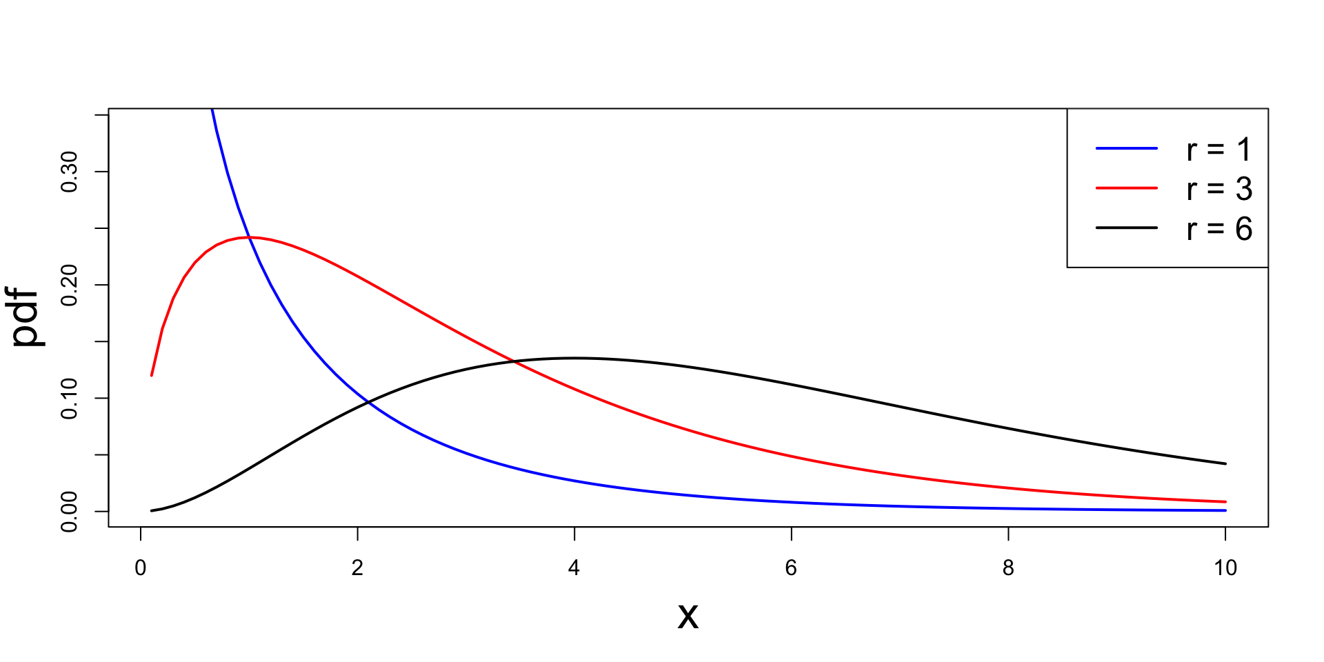
Chi-squared distribution

Plots of chi-squared pdf for different choices of r

Proof of Theorem – Case r =1

• We start with the case r=1
• Need to prove that \chi^2_1 \sim \Gamma(1/2, 1/2)
• Therefore we need to show that the pdf of \chi^2_1 is f_{\chi^2_1}(x)=\frac{x^{-1/2} \, e^{-x/2}}{\Gamma(1/2) 2^{1/2}} \,, \quad x>0

Proof of Theorem – Case r =1

• To this end, notice that by definition \chi^2_1 \sim Z^2 \,, \qquad Z \sim N(0,1)
• Hence, for x>0 we can compute cdf via \begin{align*} F_{\chi^2_1}(x) & = P(\chi^2_1 \leq x) \\ & = P(Z^2 \leq x ) \\ & = P(- \sqrt{x} \leq Z \leq \sqrt{x} ) \\ & = 2 P (0 \leq Z \leq \sqrt{x}) \end{align*} where in the last equality we used symmetry of Z around x=0

Proof of Theorem – Case r =1

• Recalling the definition of standard normal pdf we get \begin{align*} F_{\chi^2_1}(x) & = 2 P (0 \leq Z \leq \sqrt{x}) \\ & = 2 \frac{1}{\sqrt{2\pi}} \int_0^{\sqrt{x}} e^{-t^2/2} \, dt \\ & = 2 \frac{1}{\sqrt{2\pi}} G( \sqrt{x} ) \end{align*} where we set G(x) := \int_0^{x} e^{-t^2/2} \, dt

Proof of Theorem – Case r =1

• We can now compute pdf of \chi_1^2 by differentiating the cdf

• By the Fundamental Theorem of Calculus we have G'(x) = \frac{d}{dx} \left( \int_0^{x} e^{-t^2/2} \, dt \right) = e^{-x^2/2} \quad \implies \quad G'(\sqrt{x}) = e^{-x/2}

• Chain rule yields \begin{align*} f_{\chi^2_1}(x) & = \frac{d}{dx} F_{\chi^2_1}(x) = \frac{d}{dx} \left( 2 \frac{1}{\sqrt{2\pi}} G( \sqrt{x} ) \right) \\ & = 2 \frac{1}{\sqrt{2\pi}} G'( \sqrt{x} ) \frac{x^{-1/2}}{2} = \frac{x^{-1/2} e^{-x/2}}{2^{1/2} \sqrt{\pi}} \end{align*}

Proof of Theorem – Case r =1

• It is well known that \Gamma(1/2) = \sqrt{\pi}
• Hence, we conclude f_{\chi^2_1}(x) = \frac{x^{-1/2} e^{-x/2}}{2^{1/2} \sqrt{\pi}} = \frac{x^{-1/2} e^{-x/2}}{2^{1/2} \Gamma(1/2)}
• This shows \chi_1^2 \sim \Gamma(1/2,1/2)

Proof of Theorem – Case r \geq 2

• We need to prove that \chi^2_r \sim \Gamma(r/2, 1/2)

• By definition \chi^2_r \sim Z^2_1 + \ldots + Z^2_r \,, \qquad Z_i \sim N(0,1) \quad \text{iid}

• By the Theorem in Slide 46, we have Z_1,\ldots,Z_r \,\,\, \text{iid} \quad \implies \quad Z_1^2,\ldots,Z_r^2 \,\,\, \text{iid}

• Moreover, by definition, Z_i^2 \sim \chi_1^2

• Therefore, we have \chi^2_r = \sum_{i=1}^r X_i, \qquad X_i \sim \chi^2_1 \quad \text{iid}

Proof of Theorem – Case r \geq 2

• We have just proven that \chi_1^2 \sim \Gamma (1/2,1/2)

• Moreover, the Theorem in Slide 53 guarantees that Y_i \sim \Gamma(\alpha_i, \beta) \quad \text{independent} \quad \implies \quad Y_1 + \ldots + Y_n \sim \Gamma(\alpha,\beta) where \alpha = \alpha_1 + \ldots + \alpha_n

• Therefore, we conclude that \chi^2_r = \sum_{i=1}^r X_i, \qquad X_i \sim \Gamma(1/2,1/2) \quad \text{iid} \quad \implies \quad \chi^2_r \sim \Gamma(r/2,1/2)

Part 5:
Sampling from normal distribution

Sampling from Normal distribution

Sample mean and variance: For a random sample X_1,\ldots,X_n defined by S^2 := \frac{1}{n-1} \sum_{i=1}^n \left( X_i - \overline{X} \right)^2 \,, \qquad \overline{X} := \frac{1}{n} \sum_{i=1}^n X_i

Question

Assume the sample is normal X_i \sim N(\mu,\sigma^2) \,, \quad \forall \, i = 1 , \ldots, n What are the distributions of \overline{X} and S^2?

Properties of Sample Mean and Variance

Theorem

Let X_1,\ldots,X_n be a random sample from N(\mu,\sigma^2). Then

• \overline{X} and S^2 are independent random variables
• \overline{X} and S^2 are distributed as follows \overline{X} \sim N(\mu,\sigma^2/n) \,, \qquad \frac{(n-1)S^2}{\sigma^2} \sim \chi_{n-1}^2

Properties of Sample Mean and Variance

Proof of Theorem

• To prove independence of \overline{X} and S^2 we make use of the following Lemma
• Proof of this Lemma is technical and omitted
• For a proof see Lemma 5.3.3 in [1]

Lemma

Let X and Y be normal random variables. Then X \text{ and } Y \text{ independent } \quad \iff \quad {\rm Cov}(X,Y) = 0

Properties of Sample Mean and Variance

Proof of Theorem

• Note that X_i - \overline{X} and \overline{X} are normally distributed, being sums of iid normals

• Therefore, we can apply the Lemma to X_i - \overline X and \overline{X}

• To this end, recall that {\rm Var}[\overline X] = \sigma^2/n

• Also note that, by independence of X_1,\ldots,X_n {\rm Cov}(X_i,X_j) = \begin{cases} {\rm Var}[X_i] & \text{ if } \, i = j \\ 0 & \text{ if } \, i \neq j \\ \end{cases}

Properties of Sample Mean and Variance

Proof of Theorem

• Using bilinearity of covariance (i.e. linearity in both arguments) \begin{align*} {\rm Cov}(X_i - \overline X, \overline X) & = {\rm Cov}(X_i,\overline{X}) - {\rm Cov}(\overline X,\overline{X}) \\ & = \frac{1}{n} \sum_{j=1}^n {\rm Cov}(X_i,X_j) - {\rm Var}[\overline X] \\ & = \frac{1}{n} {\rm Var}[X_i] - {\rm Var}[\overline X] \\ & = \frac{1}{n} \sigma^2 - \frac{\sigma^2}{n} = 0 \end{align*}

• By the Lemma, we infer independence of X_i - \overline X and \overline X

Properties of Sample Mean and Variance

Proof of Theorem

• We have shown X_i - \overline X \quad \text{and} \quad \overline X \quad \text{independent}

• By the Theorem in Slide 46, we hence have (X_i - \overline X)^2 \quad \text{and} \quad \overline X \quad \text{independent}

• By the same Theorem we also get \sum_{i=1}^n (X_i - \overline X)^2 = (n-1)S^2 \quad \text{and} \quad \overline X \quad \text{independent}

• Again the same Theorem, finally implies independence of S^2 and \overline X

Properties of Sample Mean and Variance

Proof of Theorem

• We now want to show that \overline{X} \sim N(\mu,\sigma^2/n)

• We are assuming that X_1,\ldots,X_n are iid with {\rm I\kern-.3em E}[X_i] = \mu \,, \qquad {\rm Var}[X_i] = \sigma^2

• We have already seen in Slides 70 and 72 that, in this case, {\rm I\kern-.3em E}[\overline X] = \mu \,, \quad {\rm Var}[\overline{X}] = \frac{\sigma^2}{n}

• Sum of independent normals is normal (see the Theorem in slide 50)

• Therefore \overline{X} is normal, with mean \mu and variance \sigma^2/n

Properties of Sample Mean and Variance

Proof of Theorem

• We are left to prove that \frac{(n-1)S^2}{\sigma^2} \sim \chi_{n-1}^2
  • This is somewhat technical and we don’t actually prove it
  • For a proof see Theorem 5.3.1 in [1]
  • We however want to provide some intuition on why it holds
• Recall that the chi-squared distribution with r degrees of freedom is \chi_r^2 \sim Z_1^2 + \ldots + Z_r^2 with Z_i iid and N(0,1)

Properties of Sample Mean and Variance

Proof of Theorem

• By definition of S^2 we have \frac{(n-1)S^2}{\sigma^2} = \sum_{i=1}^n \frac{(X_i - \overline X)^2}{\sigma^2}

• If we replace the sample mean \overline X with the actual mean \mu we get the approximation \frac{(n-1)S^2}{\sigma^2} = \sum_{i=1}^n \frac{(X_i - \overline X)^2}{\sigma^2} \approx \sum_{i=1}^n \frac{(X_i - \mu)^2}{\sigma^2}

Properties of Sample Mean and Variance

Proof of Theorem

• Since X_i \sim N(\mu,\sigma^2), we have that Z_i := \frac{X_i - \mu}{\sigma} \sim N(0,1)

• Therefore \frac{(n-1)S^2}{\sigma^2} \approx \sum_{i=1}^n \frac{(X_i - \mu)^2}{\sigma^2} = \sum_{i=1}^n Z_i^2 \sim \chi_n^2

• The above is just an approximation:
  When replacing \mu with \overline X, we lose 1 degree of freedom \frac{(n-1)S^2}{\sigma^2} \sim \chi_{n-1}^2

Part 6:
t-distribution

Estimating the Mean

Problem

Estimate the mean \mu of a normal population

What to do?

• We can collect normal samples X_1, \ldots, X_n with X_i \sim N(\mu,\sigma^2)

• We then compute the sample mean \overline X := \frac{1}{n} \sum_{i=1}^n X_i

• We know that {\rm I\kern-.3em E}[\overline X] = \mu

\overline X approximates \mu

Question

How good is this approximation? How to quantify it?

Answer: We consider the Test Statistic T := \frac{\overline{X}-\mu}{\sigma/\sqrt{n}} \, \sim \,N(0,1)

• This is because \overline X \sim N(\mu,\sigma^2/n) – see Slide 101

• If \sigma is known, then the only unknown in T is \mu

T can be used to estimate \mu \quad \implies \quad Hypothesis Testing

Hypothesis testing

• Suppose that \mu=\mu_0 (this is called the null hypothesis)

• Using the data collected \mathbf{x}= (x_1,\ldots,x_n), we compute t := \frac{\overline{x}-\mu_0}{\sigma/\sqrt{n}} \,, \qquad \overline{x} = \frac{1}{n} \sum_{i=1}^n x_i

• When \mu = \mu_0, the number t is a realization of the test statistic (random variable) T = \frac{\overline{X}-\mu_0}{\sigma/\sqrt{n}} \, \sim \,N(0,1)

• Therefore, we can compute the probability of T being close to t p := P(T \approx t)

Hypothesis testing

Given the value p := P(T \approx t) we have 2 cases:

• p is small \quad \implies \quad reject the null hypothesis \mu = \mu_0
  • p small means it is unlikely to observe such value of t
  • Recall that t depends only on the data \mathbf{x}, and on our guess \mu_0
  • We conclude that our guess must be wrong \quad \implies \quad \mu \neq \mu_0
• p is large \quad \implies \quad do not reject the null hypothesis \mu = \mu_0
  • p large means that t occurs with reasonably high probability
  • There is no reason to believe our guess \mu_0 was wrong
  • But we also do not have sufficient reason to believe \mu_0 was correct

Important Remark

• The key step in Hypothesis Testing is computing p = P(T \approx t)

• This is only possible if we know the distribution of T = \frac{\overline{X}-\mu}{\sigma/\sqrt{n}}

• If we assume that the variance \sigma^2 is known, then T \sim N(0,1) and p is easily computed

Unknown variance

Problem

In general, the population variance \sigma^2 is unknown. What to do?

Idea: We can replace \sigma^2 with the sample variance S^2 = \frac{\sum_{i=1}^n X_i^2 - n \overline{X}^2}{n-1} The new test statistic is hence T := \frac{\overline{X}-\mu}{S/\sqrt{n}}

Distribution of the test statistic

Question

What is the distribution of

T := \frac{\overline{X}-\mu}{S/\sqrt{n}} \qquad ?

Answer: T has t-distribution with n-1 degrees of freedom

• This is also known as Student’s t-distribution
• Student was the pen name under which W.S. Gosset was publishing his research
• He was head brewer at Guinness, at the time the largest brewery in the world!
• Used t-distribution to study chemical properties of barley from low samples [2] (see original paper )

t-distribution

Definition

A random variable T has Student’s t-distribution with p degrees of freedom, denoted by T \sim t_p \,, if the pdf of T is f_T(t) = \frac{\Gamma \left( \frac{p+1}{2} \right) }{\Gamma \left( \frac{p}{2} \right)} \, \frac{1}{(p\pi)^{1/2}} \, \frac{ 1 }{ (1 + t^2/p)^{(p+1)/2} } \,, \qquad t \in \mathbb{R}

Characterization of the t-distribution

Theorem

Let U \sim N(0,1) and V \sim \chi_p^2 be independent random variables. Then T := \frac{U}{\sqrt{V/p}} \, \sim \, t_p \,, that is, T has t-distribution with p degrees of freedom.

Proof: Given as exercise in Homework assignments

Distribution of t-statistic

As a consequence of the Theorem in previous slide we obtain:

Theorem

Let X_1,\ldots,X_n be a random sample from N(\mu,\sigma^2). Then the random variable T = \frac{\overline{X}-\mu}{S/\sqrt{n}} has t-distribution with n-1 degrees of freedom, that is, T \sim t_{n-1}

Distribution of t-statistic

Proof of Theorem

• Since X_1,\ldots,X_n is random sample from N(\mu,\sigma^2), we have that (see Slide 101) \overline{X} \sim N(\mu, \sigma^2/n)

• Therefore, we can renormalize and obtain U := \frac{ \overline{X} - \mu }{ \sigma/\sqrt{n} } \sim N(0,1)

Distribution of t-statistic

Proof of Theorem

• We have also shown that V := \frac{ (n-1) S^2 }{ \sigma^2 } \sim \chi_{n-1}^2

• Finally, we can rewrite T as T = \frac{\overline{X}-\mu}{S/\sqrt{n}} = \frac{U}{ \sqrt{V/(n-1)} }

• By the Theorem in Slide 118, we conclude that T \sim t_{n-1}

Properties of t-distribution

Proposition: Expectation and Variance of t-distribution

Suppose that T \sim t_p. We have:

• If p>1 then {\rm I\kern-.3em E}[T] = 0
• If p>2 then {\rm Var}[T] = \frac{p}{p-2}

Notes:

• We have to assume p>1, otherwise {\rm I\kern-.3em E}[T] = \infty for p=1
• We have to assume p>2, otherwise {\rm Var}[T] = \infty for p=1,2
• {\rm I\kern-.3em E}[T] = 0 follows trivially from symmetry of the pdf f_T(t) around t=0
• Computing {\rm Var}[T] is quite involved, and we skip it

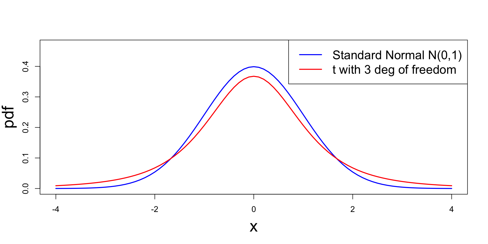
t-distribution

Comparison with Standard Normal

The t_p distribution approximates the standard normal N(0,1):

• t_p it is symmetric around zero and bell-shaped, like N(0,1)
• t_p has heavier tails compared to N(0,1)
• While the variance of N(0,1) is 1, the variance of t_p is \frac{p}{p-2}
• We have that t_p \to N(0,1) \quad \text{as} \quad p \to \infty

Plot: Comparison with Standard Normal

Part 7:
Hypothesis testing

Definition of Hypothesis

• Idea:
  • Interested in knowing a population parameter \theta
  • \theta cannot be measured directly
  • We can sample the population and draw conclusions on \theta
  • Such conclusions are called hypotheses

Definition

A hypothesis is a statement about a population parameter

Complementary hypotheses

• Two hypotheses are complementary if exactly one of them can be true

• Complementary hypotheses are called:

  • H_0 the null hypothesis
  • H_1 the alternative hypothesis

• Goal: Find a way to decide which between H_0 and H_1 is true

How to model hypotheses

We denote by:

• \theta a population parameter
• \Theta the space of all population parameters

For \Theta_0 \subset \Theta we define the associated null and alternative hypotheses as \begin{align*} H_0 \colon & \theta \in \Theta_0 & \qquad \text{ null hypothesis} \\ H_1 \colon & \theta \in \Theta_0^c & \qquad \text{ alternative hypothesis} \end{align*}

Definition of Hypothesis test

Definition

A hypothesis test is a rule to decide:

• For which sample values we decide to accept H_0 as true
• For which sample values we reject H_0 and accept H_1 as true

Acceptance and Critical regions

The sample space is partitioned into two regions:

• Acceptance region: For samples \mathbf{x} in this region we accept H_0
• Critical region: For samples \mathbf{x} in this region we reject H_0

In most cases: Critical region is defined in terms of a test statistic W(\mathbf{x})

Example: We could decide to reject H_0 if W(\mathbf{x}) \in R with R \subset \mathbb{R} some rejection region

One-sided vs Two-sided Tests

Let \theta be one dimensional parameter. A hypothesis test is:

• One-sided: if the null and alternative hypotheses are of the form H_0 \colon \theta \leq \theta_0 \,, \qquad H_1 \colon \theta > \theta_0 or also H_0 \colon \theta \geq \theta_0 \,, \qquad H_1 \colon \theta < \theta_0

• Two-sided: if the null and alternative hypotheses are of the form H_0 \colon \theta = \theta_0 \,, \qquad H_1 \colon \theta \neq \theta_0

Example 1: Two-sided test

We want to assess whether a coin is fair

• To test fairness, toss the coin many times and record outcome

• \theta = proportion of Heads

• The decision is between:

  • Null hypothesis: The coin is fair \,\, \implies \,\, \theta = \frac12
  • Alternative hypothesis: The coin is not fair \,\, \implies \,\, \theta \neq \frac12

Hypothesis test: \qquad \quad H_0 \colon \theta = \frac12 \,, \qquad H_1 \colon \theta \neq \frac12

Example 2: One-sided test

A University wants to advertise its MBA Program: \text{ MBA } = \text{ higher salary }

• Is this a true or false statement?

• The University has only access to incomplete data (could not ask all former students). Need hypothesis testing

• \theta = average change in salary after completing the MBA program

  • Null hypothesis: No improvement in salary \,\, \implies \,\, \theta \leq 0
  • Alternative hypothesis: Salary increases \,\, \implies \,\, \theta > 0

Hypothesis test: \qquad \quad H_0 \colon \theta \leq 0 \,, \qquad H_1 \colon \theta > 0

Part 8:
The one-sample t-test

One-sample Two-sided t-test

Goal: estimate the mean \mu of a normal population N(\mu,\sigma^2). If \mu_0 is guess for \mu H_0 \colon \mu = \mu_0 \qquad H_1 \colon \mu \neq \mu_0

• One-sample means we sample only from one population
• The variance \sigma is unknown
• Suppose the sample size is n, with sample X_1 ,\ldots,X_n
• We consider the t-statistics T = \frac{\overline{X}-\mu_0}{S/\sqrt{n}}
• Recall: T \sim t_{n-1} Student’s t-distribution with n-1 degrees of freedom

Procedure for all tests

1. Calculation
2. Reference statistical tables or numerical values
3. Interpretation

One-sample Two-sided t-test

Calculation

• We have n samples available x_1,\ldots,x_n
• Compute sample mean \overline{x} = \frac{1}{n} \sum_{i=1}^n x_i
• Compute the sample standard deviation s = \sqrt{\frac{\sum_{i=1}^n x_i^2 - n \overline{x}^2}{n-1}}

One-sample Two-sided t-test

Calculation

• Compute the estimated standard error \mathop{\mathrm{e.s.e.}}= \frac{s}{\sqrt{n}}

• Compute the sample t-statistic t = \frac{\text{estimate } - \text{ hypothesised value}}{\mathop{\mathrm{e.s.e.}}} = \frac{\overline x - \mu_0}{s/\sqrt{n}}

• \mu_0 is the value of the null hypothesis H_0

One-sample Two-sided t-test

p-value

• In alternative to computing the t-statistic, we can compute the p-value

• p-value is a measure of likely we are to observe the data if we assume the null hypothesis is true

• We have 2 options:

  • LOW p-value \quad \implies \quad reject H_0
  • HIGH p-value \quad \implies \quad do not reject H_0

• In this module we reject H_0 for p-values p<0.05

One-sample Two-sided t-test

p-value

• For the two-sided t-test, the p-value is defined as p := 2P(t_{n-1} > |t| \, | \, H_0) where t_{n-1} follows the t-distribution with n-1 degrees of freedom

• In other words, the p-value is p = 2P(\text{Observing values more extreme than |t| }| \, \mu=\mu_0)

One-sample Two-sided t-test

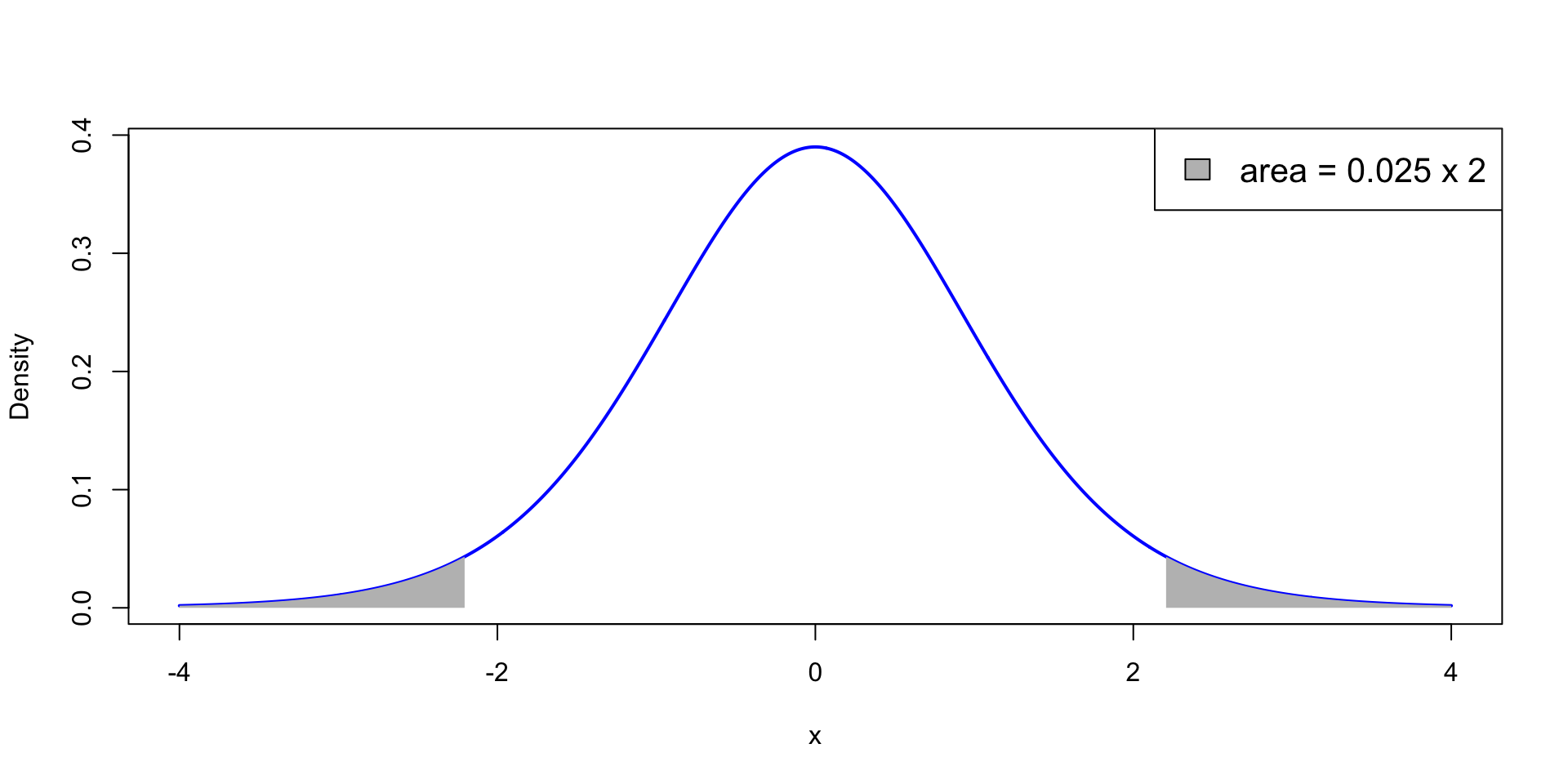
p-value

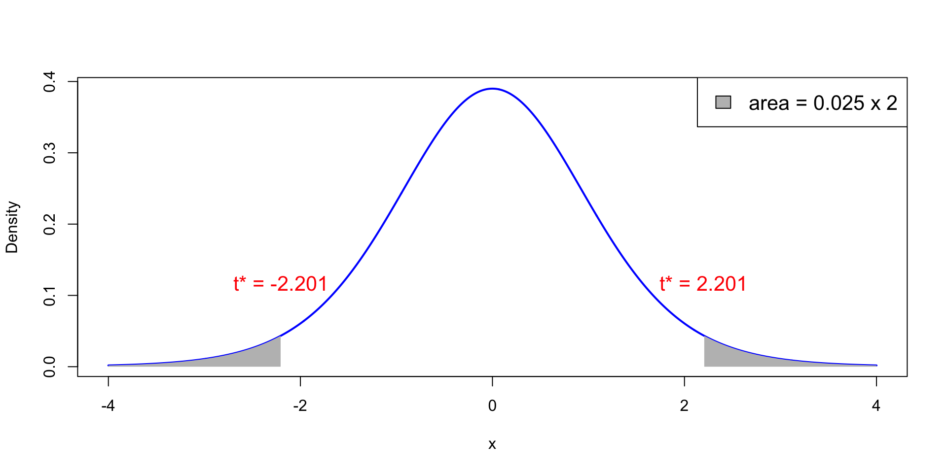
• p<0.05 means that the test statistic t is extreme: \,\, P(t_{n-1} > |t|)<0.025

• t falls in the grey areas in the t_{n-1} plot below: Each grey area measures 0.025

One-sample Two-sided t-test

p-value

• How to compute p?
  • Use statistical tables – Available here
  • Use R – Next sections

One-sample Two-sided t-test

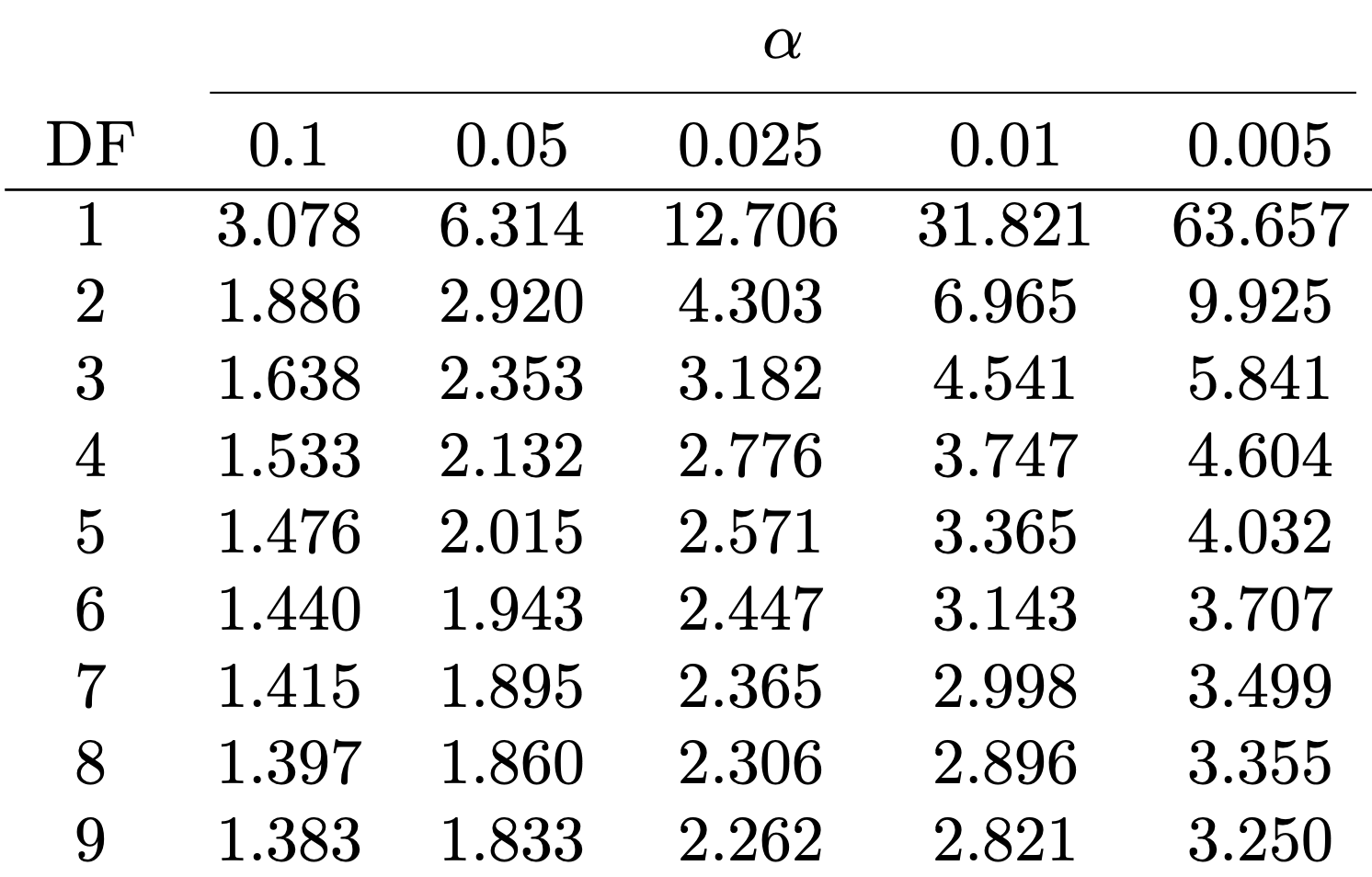
Reference statistical tables

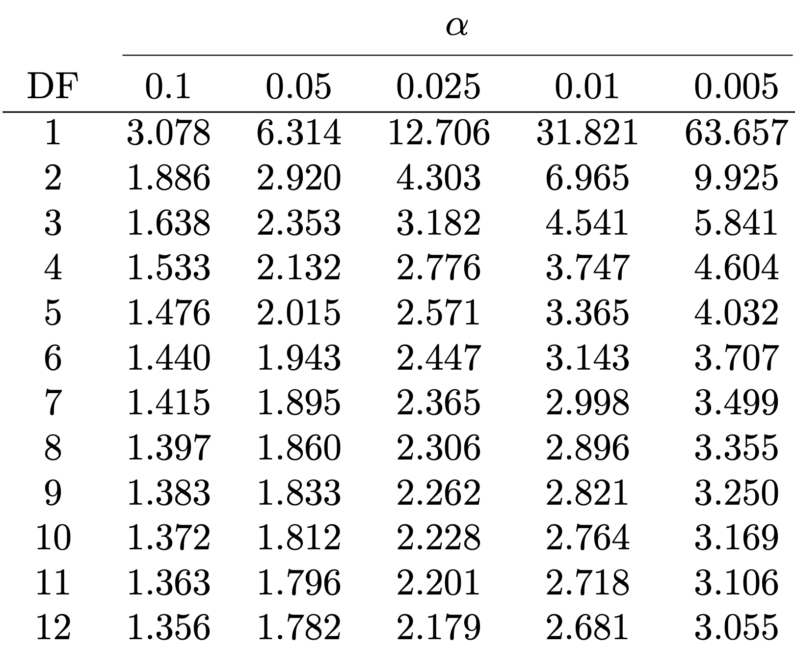
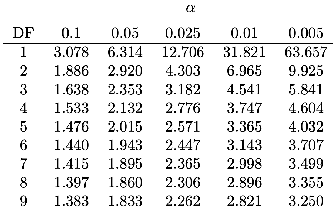
• Find Table 1 in this file

• Look at the row with Degree of Freedom n-1 (or its closest value)

• Find critical value t^* := t_{n-1}(0.025) in column \alpha = 0.025

• Example: n=10, DF =9, t^*=t_{9}(0.025)=2.262

One-sample Two-sided t-test

Reference statistical tables

• The critical value t^* = t_{n-1}(0.025) found in the table satisfies P(t_{n-1}>t^*) = 0.025

• By definition of p-value for two-sided t-test we have p := 2P(t_{n-1}>|t|)

• Therefore, for |t|>t^* \begin{align*} p & := 2P(t_{n-1}>|t|) \\ & < 2P(t_{n-1}>t^*) = 2 \cdot (0.025) = 0.05 \end{align*}

• Conclusion: \quad |t|>t^* \iff p<0.05 \qquad (Extreme t \iff low p-value)

One-sample Two-sided t-test

Interpretation

Recall that p = 2P ( \text{Observing values more extreme than t } | \mu = \mu_0)

We have two possibilities:

• |t|>t^*
  • In this case p<0.05
  • The observed statistic t is very unlikely under H_0 \,\, \implies \,\, reject H_0
• |t| \leq t^*
  • In this case p>0.05
  • The observed statistic t is not unlikely under H_0 \,\, \implies \,\, do not reject H_0

Example: 2008 crisis

• Data: Monthly Consumer Confidence Index (CCI) in 2007 and 2009
• Question: Did the crash of 2008 have lasting impact upon CCI?
• Observation: Data shows a massive drop in CCI between 2009 and 2007
• Method: Use t-test to see whether there was a change in CCI

Month	J	F	M	A	M	J	J	A	S	O	N	D
CCI 2007	86	86	88	90	99	97	97	96	99	97	90	90
CCI 2009	24	22	21	21	19	18	17	18	21	23	22	21
Difference	62	64	67	69	80	79	80	78	78	74	68	69

Example: 2008 crisis

• This is really a two-sample problem – CCI data in 2 populations: 2007 and 2009
• It reduces to a one-sample problem because we have directly comparable units
• If units cannot be compared, then we must use a two-sample approach
• Two-sample approach will be discussed later

Month	J	F	M	A	M	J	J	A	S	O	N	D
CCI 2007	86	86	88	90	99	97	97	96	99	97	90	90
CCI 2009	24	22	21	21	19	18	17	18	21	23	22	21
Difference	62	64	67	69	80	79	80	78	78	74	68	69

Setting up the test

• We want to test if there was a change in CCI from 2007 to 2009
• We are really only interested in the difference in CCI
• Let \mu be the (unknown) average difference in CCI
• The null hypothesis is that there was (on average) no change in CCI H_0 \colon \mu = 0
• The alternative hypothesis is that there was some change: H_1 \colon \mu \neq 0
• Note that this is a two-sided test

Calculation

Using the available data, we need to compute:

• Sample mean and standard deviation \overline{x} = \frac{1}{n} \sum_{i=1}^n x_i \qquad s = \sqrt{\frac{\sum_{i=1}^n x_i^2 - n \overline{x}^2}{n-1}}

• Test statistic t = \frac{\overline x - \mu_0}{s/\sqrt{n}}

Calculation

CCI	J	F	M	A	M	J	J	A	S	O	N	D
Difference	62	64	67	69	80	79	80	78	78	74	68	69

\begin{align*} \overline{x} & =\frac{1}{n} \sum_{i=1}^{n} x_i=\frac{1}{12} \left(62+64+67+{\ldots}+68+69\right)=\frac{868}{12}=72.33 \\ \sum_{i=1}^{n} x_i^2 & = 62^2+64^2+67^2+{\ldots}+68^2+69^2 = 63260 \\ s & = \sqrt{ \frac{\sum_{i=1}^n x_i^2 - n \overline{x}^2}{n-1} } = \sqrt{\frac{63260-12\left(\frac{868}{12}\right)^2}{11}} = \sqrt{\frac{474.666}{11}} = 6.5689 \end{align*}

Calculation

• The sample size is n=12
• The sample mean is \overline{x}=72.33
• The sample standard deviation is s = 6.5689
• The hypothesized mean is \mu_0 = 0
• The t-statistic is t = \frac{\overline{x} - \mu_0}{s/\sqrt{n}} = \frac{72.33 - 0}{6.5689/\sqrt{12}} = 38.145

Reference statistical tables

Find Table 1 in this file

• Find row with DF = n-1 (or closest). Find critical value t^* in column \alpha = 0.025
• In our case: n=12, DF =11, t^*= t_{11}(0.025) =2.201

Reference statistical tables

• Plot of t_{11} distribution. White area is 0.95, total shaded area is 0.05
• Probability of observing |t|>t^* = 2.201 is p<0.025

Interpretation

• We have computed:

  • Test statistic t = 38.145
  • Critical value t^* = 2.201

• Therefore |t| = 38.145 > 2.201 = t^*

• This implies rejecting the null hypothesis H_0 \colon \mu = 0

Interpretation

• t-test implies that mean difference in CCI is \mu \neq 0

• The sample mean difference is positive (\bar{x}=72.33)

• Conclusions:

  • CCI has changed from 2007 to 2009 (backed by t-test)
  • CCI seems higher in 2007 than in 2009 (backed by sample mean)
  • The 2008 crash seems to have reduced consumer confidence

One-sided t-tests

• Suppose given a hypothesized value \mu_0 for the mean \mu of a normal population

• In certain situations, if the true mean differs from \mu_0 (\mu \neq \mu_0), you may have reason to believe specifically that \mu < \mu_0 \qquad \text{or} \qquad \mu > \mu_0

• In such cases, you would support these conclusions if, respectively, t \ll 0 \qquad \text{or} \qquad t \gg 0 \, , where t is the t-statistic defined as t = \frac{\overline{x} - \mu_0}{\mathop{\mathrm{e.s.e.}}} Reject H_0 if the t-statistic is sufficiently extreme to the left OR right

Summary: The one-sample t-test

Suppose given a sample

• x_1, \ldots, x_n from N(\mu_X,\sigma^2) of size n

The two-sided hypothesis for testing if \mu = \mu_0 is H_0 \colon \mu = \mu_0 \,, \quad \qquad H_1 \colon \mu \neq \mu_0

The one-sided alternative hypotheses are H_1 \colon \mu < \mu_0 \quad \text{ or } \quad H_1 \colon \mu > \mu_0

Procedure: 3 Steps

1. Calculation: Compute the t-statistic t = \frac{ \overline{x} - \mu_0}{ s/\sqrt{n} } where \mu_0 is the null hypothesis, and sample mean and standard deviation are \overline{x} = \frac{1}{n} \sum_{i=1}^n x_i \,, \qquad s = \sqrt{\frac{\sum_{i=1}^n x_i^2 - n \overline{x}^2}{n-1} }

2. Statistical Tables or R: Find either
   • Critical value t^* in Table 1
   • p-value in R (later)

3. Interpretation: Reject H_0 when either p < 0.05 \qquad \text{ or } \qquad t \in \,\,\text{Rejection Region} \qquad \qquad \qquad \qquad (T \, \sim \, t_{n-1})

Alternative	Rejection Region	t^*	p-value
\mu \neq \mu_0	|t| > t^*	t_{n-1}(0.025)	2P(T > |t|)
\mu < \mu_0	t < - t^*	t_{n-1}(0.05)	P(T < t)
\mu > \mu_0	t > t^*	t_{n-1}(0.05)	P(T > t)

Reject H_0 if t-statistic t falls in the Rejection Region (the gray areas)

Example: Rising textbook costs

• The University Bookstore claims that, on average, a student will pay 500£ per semester for textbooks and supplies

• The Student Union does not believe the University Bookstore’s claims: They think the students spend more

• They interviewed 10 students, asking each how much they spent on textbooks and supplies. The answers are below.

Costs

304

431

385

987

303

480

455

724

642

506

To test whether the students spend more than 500£, we consider the one-sided alternative hypothesis

H_0 \colon \mu = 500 \,, \qquad H_1 \colon \mu > 500

Calculation

Costs

304

431

385

987

303

480

455

724

642

506

\begin{align*} \overline{x} & =\frac{1}{n} \sum_{i=1}^{n} x_i=\frac{1}{10} \left(304+431+{\ldots}+642+506\right)=\frac{5217}{10}=521.7 \\ \sum_{i=1}^{n} x_i^2 & = 304^2+431^2+{\ldots}+642^2+506^2 = 3122181 \\ s & = \sqrt{ \frac{\sum_{i=1}^n x_i^2 - n \overline{x}^2}{n-1} } = \sqrt{\frac{3122181-10\left(\frac{5217}{10}\right)^2}{9}} = 210.9429 \end{align*}

Calculation

• The sample size is n=10
• The sample mean is \overline{x}=521.7
• The sample standard deviation is s = 210.9429
• The hypothesized mean is \mu_0 = 500
• The t-statistic is

t = \frac{\overline{x} - \mu_0}{s/\sqrt{n}} = \frac{521.7 - 500}{210.9429/\sqrt{10}} \approx 0.325

Reference statistical tables

Find Table 1 in this file

• We are conducting a one-sided test \quad \implies \quad \alpha = 0.05

• Degrees of freedom are DF = n-1 = 9

• Therefore, the required critical value is t^*= t_{9}(0.05) = 1.833

The Rejection Region

• Plot of t_{9} distribution. White area is 0.95, gray area is 0.05

• The grey zone is the Rejection Region

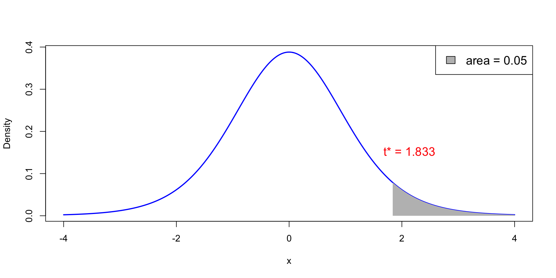
Interpretation

• We have computed:
  • Test statistic t = 0.325
  • Critical value t^* = 1.833
• Therefore, we see that t does not belong to the rejection region

t = 0.325 < 1.833 = t^*

• There is not enough evidence to reject the null hypothesis H_0 \colon \mu = 500

• Conclusion: The data gives us little reason to doubt that students spend more than 500£ per semester

References

[1]

Casella, George, Berger, Roger L., Statistical inference, second edition, Brooks/Cole, 2002.

[2]

Gosset (Student), W.S., The probable error of a mean, Biometrika. 6 (1908) 1–25.