TrSS ESS
174664.1 586719.6 Statistical Models
Lecture 11
Lecture 11:
ANOVA
Outline of Lecture 11
- One-way ANOVA
- Factors in R
- Anova with aov
- Dummy variable regression models
- ANOVA as Regression
- ANCOVA
Part 1:
One-way ANOVA
Introduction
ANOVA means Analysis of variance
Method of comparing means across samples
We first present ANOVA in the traditional way
Then we show that the ANOVA model is just a special form of linear regression
- In particular, ANOVA models can be fitted with
lm
- In particular, ANOVA models can be fitted with
One-way ANOVA
- ANOVA allows to compare population means for several independent samples
- Can be seen as generalization of t-test for two independent samples
- Suppose we have k populations of interest, with distribution N(\mu_k,\sigma^2)
- Note that the variance is the same for all populations
- Sample from population i is denoted x_{i1}, x_{i2}, \ldots , x_{in_i}
Goal: Compare population means \mu_i
Hypothesis set: We test for a difference in means
\begin{align*} H_0 \colon & \mu_1 = \mu_2 = \ldots = \mu_k \\ H_1 \colon & \mu_i \neq \mu_j \,\, \text{ for at least one pair } \, i \neq j \end{align*}
ANOVA is generalization of two-sample t-test to multiple populations
Constructing a Test statistic
- We formulate a statistic which compares
- variations within a single group to
- variations among the groups
- Denote the mean of the i-th sample by
\overline{x}_i = \frac{1}{n_i} \sum_{j=1}^{n_i} x_{ij}
- Denote the grand mean of all samples by
\overline{x} = \frac{1}{k} \sum_{i=1}^k \overline{x}_i = \frac{1}{k} \sum_{i=1}^k \left( \frac{1}{n_i} \sum_{j=1}^{n_i} x_{ij} \right)
- The total sum of squares is
\mathop{\mathrm{TSS}}:= \sum_{i=1}^{k} \sum_{j=1}^{n_i} ( x_{ij} - \overline{x} )^2
\mathop{\mathrm{TSS}} measures deviation of samples from the grand mean \overline{x}
The Error Sum of Squares is
\mathop{\mathrm{ESS}}= \sum_{i=1}^k \sum_{j=1}^{n_i} (x_{ij} - \overline{x}_i)^2
The interior sum of \mathop{\mathrm{ESS}} measures the variation within the i-th group
\mathop{\mathrm{ESS}} is then a measure of the within-group variability
- The Treatment Sum of Squares is
\mathop{\mathrm{TrSS}}= \sum_{i=1}^{k} n_i ( \overline{x}_i - \overline{x})^2
\mathop{\mathrm{TrSS}} compares the means for each group \overline{x}_i with the grand mean \overline{x}
\mathop{\mathrm{TrSS}} is then a measure of variability among the groups
Note: Treatment comes from medical experiments, where the population mean models the effect of some treatment
Proposition
The following decomposition holds
\mathop{\mathrm{TSS}}= \mathop{\mathrm{ESS}}+ \mathop{\mathrm{TrSS}}
The ANOVA F-statistic
Assume k independent populations with distributions N(\mu_i,\sigma^2)
Assume to have n_i independent samples from each population: x_{i1}, x_{i2}, \ldots, x_{in_i}
Define the total number of samples as n = \sum_{i=1}^k n_i
Define the Error and Treatment Sum of Squares as in the previous slides
\mathop{\mathrm{TrSS}}= \sum_{i=1}^{k} n_i ( \overline{x}_i - \overline{x})^2 \,, \qquad \mathop{\mathrm{ESS}}= \sum_{i=1}^k \sum_{j=1}^{n_i} (x_{ij} - \overline{x}_i)^2
Theorem
The F-statistic for the one-way ANOVA test follows an F-distribution:
F := \frac{ \mathop{\mathrm{TrSS}}}{ k - 1 } \bigg/ \frac{ \mathop{\mathrm{ESS}}}{ n - k } \ \sim \ F_{k-1,n-k}
\begin{align*} \text{Case 1: } \, H_0 \, \text{ holds } & \, \iff \, \text{Population means are all the same} \\[15pt] & \, \iff \, \text{i-th sample mean is similar to grand mean: } \, \overline{x}_i \approx \overline{x} \,, \quad \forall\, i\\[15pt] & \, \iff \, \mathop{\mathrm{TrSS}}= \sum_{i=1}^{k} n_i ( \overline{x}_i - \overline{x})^2 \approx 0 \, \iff \, F = \frac{ \mathop{\mathrm{TrSS}}}{ k - 1 } \bigg/ \frac{ \mathop{\mathrm{ESS}}}{ n - k } \approx 0 \end{align*}
\begin{align*} \text{Case 2: } \, H_1 \, \text{ holds } & \, \iff \, \text{At least two population means are different} \\[15pt] & \, \iff \, \text{At least two populations satisfy } \, (\overline{x}_i - \overline{x})^2 \gg 0 \\[15pt] & \, \iff \, \mathop{\mathrm{TrSS}}= \sum_{i=1}^{k} n_i ( \overline{x}_i - \overline{x})^2 \gg 0 \, \iff \, F = \frac{ \mathop{\mathrm{TrSS}}}{ k - 1 } \bigg/ \frac{ \mathop{\mathrm{ESS}}}{ n - k } \gg 0 \end{align*}
Therefore, the test is one-sided: \,\, Reject H_0 \iff F \gg 0
The one-way ANOVA F-test
Suppose given k independent samples
- Sample x_{i1}, \ldots, x_{in_i} i.i.d from N(\mu_i,\sigma^2)
Goal: Compare population means \mu_i
Hypothesis set: We test for a difference in means
\begin{align*} H_0 \colon & \mu_1 = \mu_2 = \ldots = \mu_k \\ H_1 \colon & \mu_i \neq \mu_j \,\, \text{ for at least one pair } \, i \neq j \end{align*}
Procedure: 3 Steps
- Calculation: Compute total number of samples, samples mean and grand mean n = \sum_{i=1}^k n_i \,, \qquad \overline{x}_i = \frac{1}{n_i} \sum_{j=1}^{n_i} x_{ij} \,, \qquad \overline{x} = \frac{1}{k} \sum_{i=1}^k \overline{x}_i Compute the \mathop{\mathrm{TrSS}} and \mathop{\mathrm{ESS}} \mathop{\mathrm{TrSS}}= \sum_{i=1}^{k} n_i ( \overline{x}_i - \overline{x})^2 \,, \qquad \mathop{\mathrm{ESS}}= \sum_{i=1}^k \sum_{j=1}^{n_i} (x_{ij} - \overline{x}_i)^2 Compute the F-statistic F = \frac{ \mathop{\mathrm{TrSS}}}{ k - 1 } \bigg/ \frac{ \mathop{\mathrm{ESS}}}{ n - k } \ \sim \ F_{k-1,n-k}
- Statistical Tables or R: Find either
- Critical value F^* in Table 3
- p-value in R
- Interpretation: Reject H_0 when either p < 0.05 \qquad \text{ or } \qquad F \in \,\,\text{Rejection Region}
| Alternative | Rejection Region | F^* | p-value |
|---|---|---|---|
| \exists \,\, i \neq j s.t. \mu_i \neq \mu_j | F > F^* | F_{k-1,n-k}(0.05) | P(F_{k-1,n-k} > F) |
Worked Example: Calorie Consumption
Consider 15 subjects split at random into 3 groups
Each group is assigned a month
For each group we record the number of calories consumed on a randomly chosen day
Assume that calories consumed are normally distributed with common variance, but maybe different means
| May | 2166 | 1568 | 2233 | 1882 | 2019 |
| Sep | 2279 | 2075 | 2131 | 2009 | 1793 |
| Dec | 2226 | 2154 | 2583 | 2010 | 2190 |
Question: Is there a difference in calories consumed each month?
Boxplot of the data
To visually compare sample means for each population
# Enter the data
may <- c(2166, 1568, 2233, 1882, 2019)
sep <- c(2279, 2075, 2131, 2009, 1793)
dec <- c(2226, 2154, 2583, 2010, 2190)

# Combine vectors into a list and label them
data <- list(May = may, September = sep, December = dec)

# Create the boxplot
boxplot(data,
        main = "Boxplot of Calories Consumed each month",
        ylab = "Daily calories consumed")
It seems that consumption is, on average, higher in colder months
We suspect population means are different: need one-way ANOVA F-test
Performing the one-way ANOVA F-test
- We first compute sample means and grand mean \overline{x}_i = \frac{1}{n_i} \sum_{j=1}^{n_i} x_{ij} \,, \qquad \overline{x} = \frac{1}{k} \sum_{i=1}^k \overline{x}_i
There are 3 groups, each with n_i = 5 samples
Compute the \mathop{\mathrm{TrSS}} and \mathop{\mathrm{ESS}} \mathop{\mathrm{TrSS}}= \sum_{i=1}^{k} n_i ( \overline{x}_i - \overline{x})^2 = 5 \sum_{i=1}^{k} ( \overline{x}_i - \overline{x})^2 \,, \qquad \mathop{\mathrm{ESS}}= \sum_{i=1}^k \sum_{j=1}^{n_i} (x_{ij} - \overline{x}_i)^2
We have k = 3 groups; \, n = 15 total samples
Compute the F-statistic
F = \frac{ \mathop{\mathrm{TrSS}}}{ k - 1 } \bigg/ \frac{ \mathop{\mathrm{ESS}}}{ n - k } \ \sim \ F_{k-1,n-k}
# Enter number of groups and sample size
k <- 3; n <- 15

# Compute F-statistic
F.obs = ( TrSS/(k-1) ) / ( ESS/(n-k) )

# Print
F.obs
[1] 1.786177- Compute the p-value
p = P( F_{k-1,n-k} > F ) = 1 - P( F_{k-1,n-k} \leq F )
[1] 0.2093929The p-value is p > 0.05 \quad \implies \quad Do not reject H_0
No reason to believe that population means are different
Conclusion: Despite the boxplot, the variation in average monthly calories consumption can be explained by chance only
Next: Use native R command for ANOVA test - Need Factors
Part 2:
Factors in R
Factors in R
Factors: A way to represent discrete variables taking a finite number of values
Example: Suppose to have a vector of people’s names
- Let us store the sex of each person as either
- Numbers: \, \texttt{1} represents female and \texttt{0} represents male
- Strings: \, \texttt{"female"} and \texttt{"male"}
The factor command
- The \, \texttt{factor} command turns a vector into a factor
sex.num <- c(1, 1, 1, 0, 1, 0)

# Turn sex.num into a factor
sex.num.factor <- factor(sex.num)

# Print the factor obtained
print(sex.num.factor)
[1] 1 1 1 0 1 0
Levels: 0 1The factor \, \texttt{sex.num.factor} looks like the original vector \, \texttt{sex.num}
The difference is that the factor \, \texttt{sex.num.factor} contains levels
- In this case the levels are \, \texttt{0} and \, \texttt{1}
- Levels are all the (discrete) values assumed by the vector \, \texttt{sex.num}
The factor command
- In the same way we can convert \, \texttt{sex.char} into a factor
sex.char <- c("female", "female", "female", "male", "female", "male")
# Turn sex.char into a factor
sex.char.factor <- factor(sex.char)
# Print the factor obtained
print(sex.char.factor)[1] female female female male female male
Levels: female maleAgain, the factor \, \texttt{sex.char.factor} looks like the original vector \, \texttt{sex.char}
Again, the difference is that the factor \, \texttt{sex.char.factor} contains levels
- In this case the levels are strings \, \texttt{"female"} and \, \texttt{"male"}
- These 2 strings are all the values assumed by the vector \, \texttt{sex.char}
Reordering the Levels
- Factor levels are automatically ordered by R
- Increasing order for numerical factors; Alphabetical order for string factors
- We can manually reorder the factor levels. For example, compare:
sex.char <- c("female", "female", "female", "male", "female", "male")
# Turn sex.char into a factor
factor(sex.char)[1] female female female male female male
Levels: female male[1] female female female male female male
Levels: male femaleSubsetting factors
- Factors can be subsetted exactly like vectors
[1] 1 1 1 0 1 0
Levels: 0 1[1] 1 1 0 1
Levels: 0 1Subsetting factors
- Warning: After subsetting a factor, all defined levels are still stored
- This is true even if some of the levels are no longer represented in the subsetted factor
[1] female female female male   female male
Levels: female male[1] female female female female
Levels: female maleThe levels of
sex.char.factor[c(1:3, 5)]are still \, \texttt{"female"} and \, \texttt{"male"}This is despite
sex.char.factor[c(1:3, 5)]only containing \, \texttt{"female"}
The levels function
- The levels of a factor can be extracted with the function \, \texttt{levels}
[1] "female" "male" - Note: Levels of a factor are always stored as strings, even if originally numbers
[1] "0" "1"The levels of \, \texttt{sex.num.factor} are the strings \, \texttt{"0"} and \, \texttt{"1"}
This is despite the original vector \, \texttt{sex.num} being numeric
The command \, \texttt{factor} converted numeric levels into strings
Relabelling a factor
The function \, \texttt{levels} can also be used to relabel factors
For example we can relabel
- \, \texttt{female} into \, \texttt{f}
- \, \texttt{male} into \, \texttt{m}
# Relabel levels of sex.char.factor
levels(sex.char.factor) <- c("f", "m")

# Print relabelled factor
print(sex.char.factor)
[1] f f f m f m
Levels: f mLogical subsetting of factors
Logical subsetting is done exactly like in the case of vectors
Important: Need to remember that levels are always strings
Example: To identify all the men in \, \texttt{sex.num.factor} we do
[1] FALSE FALSE FALSE TRUE FALSE TRUE- To retrieve names of men stored in \, \texttt{firstname} use logical subsetting
firstname <- c("Liz", "Jolene", "Susan", "Boris", "Rochelle", "Tim")

firstname[ sex.num.factor == "0" ]
[1] "Boris" "Tim" Part 3:
ANOVA with aov
Anova with aov
- We have conducted the one-way ANOVA F-test by hand
- This is cumbersome with large datasets with many populations
- The quick way in R is to use the command
aov(analysis of variance)
Method
Place all the samples into one long vector
valuesCreate a vector with corresponding group labels
indTurn
indinto a factorCombine
valuesandindinto a dataframedTherefore, dataframe
dcontains:- First Column: values for each sample
- Second Column: ind, indicating the group the corresponding sample is from
The ANOVA F-test is performed with
\text{aov(values } \sim \text{ ind, data = d)}
values ~ indis the formula coupling values to the corresponding group
Example 1: Calorie Consumption
Recall: we have 15 subjects split at random into 3 groups
Each group is assigned a month
For each group we record the number of calories consumed on a randomly chosen day
Assume that calories consumed are normally distributed with common variance, but maybe different means
| May | 2166 | 1568 | 2233 | 1882 | 2019 |
| Sep | 2279 | 2075 | 2131 | 2009 | 1793 |
| Dec | 2226 | 2154 | 2583 | 2010 | 2190 |
Question: Is there a difference in calories consumed each month?
Preparing the data
# Enter the data
may <- c(2166, 1568, 2233, 1882, 2019)
sep <- c(2279, 2075, 2131, 2009, 1793)
dec <- c(2226, 2154, 2583, 2010, 2190)

# Combine values into one long vector
values <- c(may, sep, dec)

# Create vector of group labels
ind <- rep(c("May", "Sep", "Dec"), each = 5)

# Turn vector of group labels into a factor
# Note that we order the levels
ind <- factor(ind, levels = c("May", "Sep", "Dec"))

# Combine values and labels into a data frame
d <- data.frame(values, ind)

# Print d for visualization
print(d)
values ind
1 2166 May
2 1568 May
3 2233 May
4 1882 May
5 2019 May
6 2279 Sep
7 2075 Sep
8 2131 Sep
9 2009 Sep
10 1793 Sep
11 2226 Dec
12 2154 Dec
13 2583 Dec
14 2010 Dec
15 2190 DecBoxplot of the data
Previously, we constructed a boxplot by placing the data into a list
Now that we have a dataframe, the commands are much simpler:
- Pass the dataframe
dtoboxplot - Pass the formula
values ~ ind
- Pass the dataframe
Already observed: Consumption is, on average, higher in colder months
We suspect population means are different: need one-way ANOVA F-test
We have already conducted the test by hand. We now use
aov
Calling aov
- Data is stored in dataframe
d- 1st column
valuescontains calories consumed - 2nd column
indcontains month labels
- 1st column
# Perform ANOVA F-test for difference in means
model <- aov(values ~ ind, data = d)

# Print summary
summary(model)
Df Sum Sq Mean Sq F value Pr(>F)
ind 2 174664 87332 1.786 0.209
Residuals 12 586720 48893 As obtained with hand calculation, the p-value is p = 0.209
p > 0.05 \implies Do not reject H_0: Population means are similar
Example 2: ANOVA vs Two-sample t-test
When only 2 groups are present, they coincide:
ANOVA F-test for difference in means
Two-sample t-test for difference in means
(with assumption of equal variance)
Example: Let us compare calories data only for the months of May and Dec
| May | 2166 | 1568 | 2233 | 1882 | 2019 |
| Dec | 2226 | 2154 | 2583 | 2010 | 2190 |
- First, let us conduct a two-sample t-test for difference in means
# Enter the data
may <- c(2166, 1568, 2233, 1882, 2019)
dec <- c(2226, 2154, 2583, 2010, 2190)

# Two-sample t-test for difference in means
t.test(may, dec, var.equal = T)$p.value
[1] 0.1259272The p-value is p \approx 0.126
Since p > 0.05, we do not reject H_0
In particular, we conclude that populations means are similar:
- Calories consumed in May and December do not differ on average
- Let us now compare the two population means with the ANOVA F-test
# Combine values into one long vector
values <- c(may, dec)

# Create factor of group labels
ind <- factor(rep(c("May", "Dec"), each = 5))

# Combine values and labels into a data frame
d <- data.frame(values, ind)

# Perform ANOVA F-test
model <- aov(values ~ ind, data = d)

# Print summary
summary(model)
Df Sum Sq Mean Sq F value Pr(>F)
ind 1 167702 167702 2.919 0.126
Residuals 8 459636 57455 The p-values p \approx 0.126 coincide! ANOVA F-test and Two-sample t-test are equivalent
This fact is discussed in details in the next 2 Parts
Part 4:
Dummy variable
Regression
Explaining the terminology
Dummy variable: Variables X which are qualitative in nature
ANOVA: refers to situations where regression models contain
- only dummy variables X
- This generalizes the ANOVA F-test seen earlier
ANCOVA: refers to situations where regression models contain a combination of
- dummy variables and quantitative (the usual) variables
Dummy variables
Dummy variable:
- A variable X which is qualitative in nature
- Often called cathegorical variables
Regression models can include dummy variables
Qualitatitve binary variables can be represented by X with
- X = 1 \, if effect present
- X = 0 \, if effect not present
Examples of binary quantitative variables are
- On / Off
- Yes / No
- Sample is from Population A / B
Dummy variables
- Dummy variables can also take several values
- These values are often called levels
- Such variables are represented by X taking discrete values
- Examples of dummy variables with several levels
- Month: Jan, Feb, Mar, …
- Season: Summer, Autumn, Winter, Spring
- Priority: Low, Medium, High
- Quarterly sales data: Q1, Q2, Q3, Q4
- UK regions: East Midlands, London Essex, North East/Yorkshire, …
Example: Fridge sales data
- Consider the dataset on quarterly fridge sales fridge_sales.txt
- Each entry represents sales data for 1 quarter
- 4 consecutive entries represent sales data for 1 year
   fridge.sales durable.goods.sales q1 q2 q3 q4 quarter
1          1317               252.6  1  0  0  0       1
2          1615               272.4  0  1  0  0       2
3          1662               270.9  0  0  1  0       3
4          1295               273.9  0  0  0  1       4
5          1271               268.9  1  0  0  0       1
6          1555               262.9  0  1  0  0       2
7          1639               270.9  0  0  1  0       3
8          1238               263.4  0  0  0  1       4
9          1277               260.6  1  0  0  0       1
10         1258               231.9  0  1  0  0       2
11         1417               242.7  0  0  1  0       3
12         1185               248.6  0  0  0  1       4
13         1196               258.7  1  0  0  0       1
14         1410               248.4  0  1  0  0       2
15         1417               255.5  0  0  1  0       3
16          919               240.4  0  0  0  1       4
17          943               247.7  1  0  0  0       1
18         1175               249.1  0  1  0  0       2
19         1269               251.8  0  0  1  0       3
20          973               262.0  0  0  0  1       4
21         1102               263.3  1  0  0  0       1
22         1344               280.0  0  1  0  0       2
23         1641               288.5  0  0  1  0       3
24         1225               300.5  0  0  0  1       4
25         1429               312.6  1  0  0  0       1
26         1699               322.5  0  1  0  0       2
27         1749               324.3  0  0  1  0       3
28         1117               333.1  0  0  0  1       4
29         1242               344.8  1  0  0  0       1
30         1684               350.3  0  1  0  0       2
31         1764               369.1  0  0  1  0       3
32 1328 356.4 0 0 0 1 4- Below are the first 4 entries of the Fridge sales dataset
- These correspond to 1 year of sales data
- First two variables are quantitative
- Fridge Sales = total quarterly fridge sales (in million $)
- Duarable Goods Sales = total quarterly durable goods sales (in billion $)
- Remaining variables are qualitative:
- Q1, Q2, Q3, Q4 \, take values 0 / 1 \quad (representing 4 yearly quarters)
- Quarter \, takes values 1 / 2 / 3 / 4 \quad (equivalent representation of quarters)
| Fridge Sales | Durable Goods Sales | Q1 | Q2 | Q3 | Q4 | Quarter |
|---|---|---|---|---|---|---|
| 1317 | 252.6 | 1 | 0 | 0 | 0 | 1 |
| 1615 | 272.4 | 0 | 1 | 0 | 0 | 2 |
| 1662 | 270.9 | 0 | 0 | 1 | 0 | 3 |
| 1295 | 273.9 | 0 | 0 | 0 | 1 | 4 |
Encoding Quarter in regression model
Two alternative approaches:
- Include 4-1 = 3 dummy variables with values 0 / 1
- Each dummy variable represents 1 Quarter
- We need 3 variables to represent 4 Quarters (plus the intercept)
- Include one variable which takes values 1 / 2 / 3 / 4
Differences between the two approaches:
This method works with command
lmThis method works with the command
aov
The dummy variable trap
- Suppose you follow the first approach:
- Encode each quarter with a separate variable
- If you have 4 different levels, you would need
- 4-1=3 dummy variables
- the intercept term
- In general: if you have k different levels, you would need
- k-1 dummy variables
- the intercept term
Question: Why only k - 1 dummy variables?
Answer: To avoid the dummy variable trap
Example: Dummy variable trap
To illustrate the dummy variable trap, consider the following
- Encode each Quarter with one dummy variable \mathbf{1}_i
\mathbf{1}_j(i) = \begin{cases} 1 & \text{ if sample i belongs to Quarter j} \\ 0 & \text{ otherwise} \\ \end{cases}
- Consider the regression model with intercept
Y = \beta_0 \cdot (1) + \beta_1 \mathbf{1}_1 + \beta_2 \mathbf{1}_2 + \beta_3 \mathbf{1}_3 + \beta_4 \mathbf{1}_4 + \varepsilon
- In the above, Y is the quartely Fridge sales data
- Each data entry belongs to exactly one Quarter. Thus
\mathbf{1}_1 + \mathbf{1}_2 + \mathbf{1}_3 + \mathbf{1}_4 = 1
Dummy variable trap: Variables are collinear (linearly dependent)
Indeed the design matrix is
Z = \left( \begin{array}{ccccc} 1 & 1 & 0 & 0 & 0 \\ 1 & 0 & 1 & 0 & 0 \\ 1 & 0 & 0 & 1 & 0 \\ 1 & 0 & 0 & 0 & 1 \\ 1 & 1 & 0 & 0 & 0 \\ \dots & \dots & \dots & \dots & \dots \\ \end{array} \right)
- First column is the sum of remaining columns \quad \implies \quad Multicollinearity
Example: Avoiding dummy variable trap
We want to avoid Multicollinearity (or dummy variable trap)
How? Drop one dummy variable (e.g. the first) and consider the model
Y = \beta_1 \cdot (1) + \beta_2 \mathbf{1}_2 + \beta_3 \mathbf{1}_3 + \beta_4 \mathbf{1}_4 + \varepsilon
If data belongs to Q1, then \mathbf{1}_2 = \mathbf{1}_3 = \mathbf{1}_4 = 0
Therefore, in general, we have
\mathbf{1}_2 + \mathbf{1}_3 + \mathbf{1}_4 \not\equiv 1
- This way we avoid Multicollinearity \quad \implies \quad no trap!
- Question: How do we interpret the coefficients in the model
Y = \beta_1 \cdot (1) + \beta_2 \mathbf{1}_2 + \beta_3 \mathbf{1}_3 + \beta_4 \mathbf{1}_4 + \varepsilon\qquad ?
- Answer: Recall the relationship
\mathbf{1}_1 + \mathbf{1}_2 + \mathbf{1}_3 + \mathbf{1}_4 = 1
- Substituting in the regression model we get
\begin{align*} Y & = \beta_1 \cdot ( \mathbf{1}_1 + \mathbf{1}_2 + \mathbf{1}_3 + \mathbf{1}_4 ) + \beta_2 \mathbf{1}_2 + \beta_3 \mathbf{1}_3 + \beta_4 \mathbf{1}_4 + \varepsilon\\[10pts] & = \beta_1 \mathbf{1}_1 + (\beta_1 + \beta_2) \mathbf{1}_2 + (\beta_1 + \beta_3) \mathbf{1}_3 + (\beta_1 + \beta_4 ) \mathbf{1}_4 + \varepsilon \end{align*}
Therefore, the regression coefficients are such that
| Group | Increase Described By |
|---|---|
| \mathbf{1}_1 | \beta_1 |
| \mathbf{1}_2 | \beta_1 + \beta_2 |
| \mathbf{1}_3 | \beta_1 + \beta_3 |
| \mathbf{1}_4 | \beta_1 + \beta_4 |
Conclusion: When fitting regression model with dummy variables
Increase for first dummy variable \mathbf{1}_1 is intercept term \beta_1
Increase for successive dummy variables \mathbf{1}_i with i > 1 is computed by \beta_1 + \beta_i
Intercept coefficient acts as base reference point
General case: Dummy variable trap
- Suppose to have a qualitative variable X which takes k different levels
- E.g. the previous example has k = 4 quarters
- Encode each level of X in one dummy variable \mathbf{1}_j
\mathbf{1}_j(i) = \begin{cases} 1 & \text{ if } X(i) = j \\ 0 & \text{ otherwise} \\ \end{cases}
- To each data entry corresponds one and only one level of X, so that
\mathbf{1}_1 + \mathbf{1}_2 + \ldots + \mathbf{1}_k = 1
- Hence Multicollinearity if intercept is present \, \implies \, Dummy variable trap!
General case: Avoid the trap!
- We drop the first dummy variable \mathbf{1}_1 and consider the model
Y = \beta_1 \cdot (1) + \beta_2 \mathbf{1}_2 + \beta_3 \mathbf{1}_3 + \ldots + \beta_k \mathbf{1}_k + \varepsilon
- For data points such that X = 1, we have
\mathbf{1}_2 = \mathbf{1}_3 = \ldots = \mathbf{1}_k = 0
- Therefore, in general, we get
\mathbf{1}_2 + \mathbf{1}_3 + \ldots + \mathbf{1}_k \not \equiv 1
- This way we avoid Multicollinearity \quad \implies \quad no trap!
General case: Interpret the output
- How to interpret the coefficients in the model
Y = \beta_1 \cdot (1) + \beta_2 \mathbf{1}_2 + \beta_3 \mathbf{1}_3 + \ldots + \beta_k \mathbf{1}_k + \varepsilon\quad ?
- We can argue similarly to the case m = 4 and use the constraint
\mathbf{1}_1 + \mathbf{1}_2 + \ldots + \mathbf{1}_k = 1
- Substituting in the regression model we get
Y = \beta_1 \mathbf{1}_1 + (\beta_1 + \beta_2) \mathbf{1}_2 + \ldots + (\beta_1 + \beta_k) \mathbf{1}_k + \varepsilon
Conclusion: When fitting regression model with dummy variables
| Group | Increase Described By |
|---|---|
| \mathbf{1}_1 | \beta_1 |
| \mathbf{1}_i | \beta_1 + \beta_i |
Increase for first dummy variable \mathbf{1}_1 is intercept term \beta_1
Increase for successive dummy variables \mathbf{1}_i with i > 1 is computed by \beta_1 + \beta_i
Intercept coefficient acts as base reference point
Part 5:
ANOVA as Regression
ANOVA F-test and regression
ANOVA can be seen as linear regression problem, by using dummy variables
In particular, we will show that
- ANOVA F-test is equivalent to F-test for overall significance
- We have already seen a particular instance of this fact in the Homework
- Simple linear regression can be used to perform two-sample t-test
(recall that two-sample t-test is just the ANOVA F-test with two populations)
- Simple linear regression can be used to perform two-sample t-test
- This was done by considering the model
Y_i = \beta_1 + \beta_2 \, \mathbf{1}_2 (i) + \varepsilon_i
Simple regression for two-sample t-test
Assume given two independent normal populations N(\mu_1, \sigma^2) and N(\mu_2, \sigma^2)
We have two samples
- Sample of size n_1 iid from population 1 a = (a_1, \ldots, a_{n_1})
- Sample of size n_2 iid from population 2 b = (b_1, \ldots, b_{n_2})
The data vector y is obtained by concatenating a and b
y = (a,b) = (a_1, \ldots, a_{n_1}, b_1, \ldots, b_{n_2} )
- We then considered the dummy variable model
Y_i = \beta_1 + \beta_2 \, \mathbf{1}_2 (i) + \varepsilon_i
- Here \mathbf{1}_2 (i) is the dummy variable relative to population B
\mathbf{1}_2(i) = \begin{cases} 1 & \text{ if i-th sample belongs to population 2} \\ 0 & \text{ otherwise} \end{cases}
- The regression function is therefore
{\rm I\kern-.3em E}[Y | \mathbf{1}_2 = x] = \beta_1 + \beta_2 x
- By construction, we have that
Y | \text{sample belongs to population 1} \ \sim \ N(\mu_1, \sigma^2)
- Therefore, by definition of \mathbf{1}_2, we get
{\rm I\kern-.3em E}[Y | \mathbf{1}_2 = 0] = {\rm I\kern-.3em E}[Y | \text{ sample belongs to population 1}] = \mu_1
- On the other hand, the regression function is
{\rm I\kern-.3em E}[Y | \mathbf{1}_2 = x] = \beta_1 + \beta_2 x
- Thus
{\rm I\kern-.3em E}[Y | \mathbf{1}_2 = 0] = \beta_1 + \beta_2 \cdot 0 = \beta_1 \qquad \implies \qquad \beta_1 = \mu_1
- Similarly, by construction, we have that
Y | \text{sample belongs to population 2} \ \sim \ N(\mu_2, \sigma^2)
- Therefore, by definition of \mathbf{1}_2, we get
{\rm I\kern-.3em E}[Y | \mathbf{1}_2 = 1] = {\rm I\kern-.3em E}[Y | \text{ sample belongs to population 2}] = \mu_2
- On the other hand, the regression function is
{\rm I\kern-.3em E}[Y | \mathbf{1}_2 = x] = \beta_1 + \beta_2 x
- Thus
{\rm I\kern-.3em E}[Y | \mathbf{1}_2 = 1] = \beta_1 + \beta_2 \qquad \implies \qquad \beta_1 + \beta_2 = \mu_2
- Therefore, we have proven
\beta_1 = \mu_1 \,, \qquad \beta_1 + \beta_2 = \mu_2 \qquad \implies \qquad \beta_2 = \mu_2 - \mu_1
- Recall the the regression model is
Y_i = \beta_1 + \beta_2 \, \mathbf{1}_{2} (i) + \varepsilon_i
- The hypothesis for F-test for Overall Significance for above model is
H_0 \colon \beta_2 = 0 \,, \qquad H_1 \colon \beta_2 \neq 0
Since \beta_2 = \mu_2 - \mu_1, the above hypothesis is equivalent to H_0 \colon \mu_1 = \mu_2 \,, \qquad H_1 \colon \mu_1 \neq \mu_2
Hypotheses for F-test of Overall Significance and two-sample t-test are equivalent
In the Homework, we have also proven that the ML estimators for the model Y_i = \beta_1 + \beta_2 \, \mathbf{1}_{2} (i) + \varepsilon_i satisfy \hat{\beta}_1 = \overline{a} \,, \qquad \hat{\beta}_2 = \overline{b} - \overline{a}
With this information, it is easy to check that they are equivalent
- F-statistic for Overall Significance
- t-statistic for two-sample t-test
F-test of Overall Significance and two-sample t-test are equivalent
- In particular, the (fitted) dummy variable regression model is
\begin{align*} Y_i & = \hat{\beta}_1 + \hat{\beta}_2 \, \mathbf{1}_{2} (i) + \varepsilon_i \\[10pt] & = \overline{a} + (\overline{b} - \overline{a}) \, \mathbf{1}_{2} (i) + \varepsilon_i \end{align*}
- Therefore, the predictions are:
\begin{align*} {\rm I\kern-.3em E}[Y| \text{Sample is from population 1}] & = \overline{a} \\[10pt] {\rm I\kern-.3em E}[Y| \text{Sample is from population 2}] & = \overline{b} \end{align*}
ANOVA F-test and Regression
Now, consider the general ANOVA case
- Assume given k independent populations with normal distribution N(\mu_i,\sigma^2)
- Example: In Fridge sales example we have k = 4 populations (the 4 quarters)
- The ANOVA hypothesis for difference in populations means is
\begin{align*} H_0 & \colon \mu_1 = \mu_2 = \ldots = \mu_k \\ H_1 & \colon \mu_i \neq \mu_j \text{ for at least one pair i and j} \end{align*}
- Goal: Show the ANOVA F-test for above hypothesis can be obtained with regression
We want to introduce dummy variable regression model which models ANOVA
To each population, associate a dummy variable \mathbf{1}_{i}(j) = \begin{cases} 1 & \text{ if j-th sample belongs to population i} \\ 0 & \text{ otherwise} \\ \end{cases}
Denote by x_{i1}, \ldots, x_{in_i} the iid sample of size n_{i} from population i
Concatenate these samples into a long vector (length n_1 + \ldots + n_2) y = (\underbrace{x_{11}, \ldots, x_{1n_1}}_{\text{population 1}}, \, \underbrace{x_{21}, \ldots, x_{2n_2}}_{\text{population 2}} , \, \ldots, \, \underbrace{x_{k1}, \ldots, x_{kn_k}}_{\text{population k}})
Consider the dummy variable model (with \mathbf{1}_{1} omitted) Y_i = \beta_1 + \beta_2 \, \mathbf{1}_{2} (i) + \beta_3 \, \mathbf{1}_{3} (i) + \ldots + \beta_k \, \mathbf{1}_{k} (i) + \varepsilon_i
In particular, the regression function is {\rm I\kern-.3em E}[Y | \mathbf{1}_{2} = x_2 , \, \ldots, \, \mathbf{1}_{k} = x_k ] = \beta_1 + \beta_2 \, x_2 + \ldots + \beta_k \, x_k
By construction, we have that Y | \text{sample belongs to population i} \ \sim \ N(\mu_i , \sigma^2)
A sample point belongs to population 1 if and only if \mathbf{1}_{2} = \mathbf{1}_{3} = \ldots = \mathbf{1}_{k} = 0
Hence, we can compute the conditional expectation {\rm I\kern-.3em E}[ Y | \mathbf{1}_{2} = 0 , \, \ldots, \, \mathbf{1}_{k} = 0] = {\rm I\kern-.3em E}[Y | \text{sample belongs to population 1}] = \mu_1
On the other hand, by definition of regression function, we get {\rm I\kern-.3em E}[ Y | \mathbf{1}_{2} = 0 , \, \ldots, \, \mathbf{1}_{k} = 0] = \beta_1 + \beta_2 \cdot 0 + \ldots + \beta_k \cdot 0 = \beta_1 \quad \implies \quad \mu_1 = \beta_1
Similarly, a sample point belongs to population 2 if and only if \mathbf{1}_{2} = 1 \quad \text{and} \quad \mathbf{1}_{1} = \mathbf{1}_{3} = \ldots = \mathbf{1}_{k} = 0
Hence, we can compute the conditional expectation {\rm I\kern-.3em E}[ Y | \mathbf{1}_{2} = 1 , \, \mathbf{1}_{3} = 0, \, \ldots, \, \mathbf{1}_{k} = 0] = {\rm I\kern-.3em E}[Y | \text{sample belongs to population } A_2] = \mu_2
On the other hand, by definition of regression function, we get {\rm I\kern-.3em E}[ Y | \mathbf{1}_{2} = 1 , \, \mathbf{1}_{3} = 0, \, \ldots, \, \mathbf{1}_{k} = 0] = \beta_1 + \beta_2 \cdot 1 + \ldots + \beta_k \cdot 0 = \beta_1 + \beta_2
Therefore, we conclude that \mu_2 = \beta_1 + \beta_2
Arguing in a similar way, we can show that \mu_i = \beta_1 + \beta_i \,, \quad \forall \, i \geq 2
Therefore, we have proven \mu_1 = \beta_1 \,, \quad \mu_i = \beta_1 + \beta_i \quad \forall \, i \geq 2 \quad \, \implies \quad \, \beta_1 = \mu_1 \,, \quad \beta_i = \mu_i - \mu_1 \quad \forall \, \, i \geq 2
Recall that the regression model is Y_i = \beta_1 + \beta_2 \, \mathbf{1}_{2} (i) + \ldots + \beta_k \, \mathbf{1}_{k} (i) + \varepsilon_i
The hypothesis for F-test for Overall Significance for above model is H_0 \colon \beta_2 = \beta_3 = \ldots = \beta_k = 0 \,, \qquad H_1 \colon \exists \, i \in \{2, \ldots, k\} \text{ s.t. } \beta_i \neq 0
Since \beta_i = \mu_i - \mu_1 for all i \geq 2, the above is equivalent to H_0 \colon \mu_1 = \mu_2 = \ldots = \mu_k \, \qquad H_1 \colon \mu_i \neq \mu_j \text{ for at least one pair } i \neq j
Hypotheses for F-test of Overall Significance and ANOVA F-test are equivalent
Denote by \overline{x}_i the mean of the sample x_{i1}, \ldots, x_{i n_i} from population i
It is easy to prove that the ML estimators for the model Y_i = \beta_1 + \beta_2 \, \mathbf{1}_{2} (i) + \ldots + \beta_k \, \mathbf{1}_{k} (i) + \varepsilon_i satisfy \hat{\beta}_1 = \overline{x}_1 \,, \qquad \hat{\beta}_i = \overline{x}_i - \overline{x}_1 \, \quad \forall \, i \geq 2
With this information, it is easy to check that they are equivalent
- F-statistic for Overall Significance
- F-statistic for ANOVA F-test
F-test of Overall Significance and ANOVA F-test are equivalent
- In particular, the (fitted) dummy variable regression model is
\begin{align*} Y_i & = \hat{\beta}_1 + \hat{\beta}_2 \, \mathbf{1}_{2} (i) + \hat{\beta}_k \, \mathbf{1}_{k} (i) + \varepsilon_i \\[10pt] & = \overline{x}_1 + (\overline{x}_2 - \overline{x}_1) \, \mathbf{1}_{2} (i) + \ldots + (\overline{x}_k - \overline{x}_1) \, \mathbf{1}_{k} (i) + \varepsilon_i \end{align*}
- Therefore, the predictions are:
{\rm I\kern-.3em E}[Y| \text{Sample is from population i}] = \hat{\beta}_1 + \hat{\beta}_i = \overline{x}_i
Worked Example
The data in fridge_sales.txt links
- Sales of fridges and Sales of durable goods
- to the time of year (Quarter)
For the moment, ignore the data on the Sales of durable goods
Goal: Determine if Fridge sales are linked to the time of the year
There are two ways this can be achieved in R
- ANOVA F-test for equality of means – using the command \, \texttt{aov}
- Dummy variable regression approach – using the command \, \texttt{lm}
- Code for this example is available here anova.R
- Data is in the file fridge_sales.txt
- We read the data into a data-frame as usual
- The first 4 rows of the data-set are given below
# Load dataset on Fridge Sales
d <- read.table(file = "fridge_sales.txt", header = TRUE)

# Print first 4 rows
head(d, n=4)
fridge.sales durable.goods.sales q1 q2 q3 q4 quarter
1 1317 252.6 1 0 0 0 1
2 1615 272.4 0 1 0 0 2
3 1662 270.9 0 0 1 0 3
4 1295 273.9 0 0 0 1 4- Quantitative variables
- Fridge sales
- Durable goods sales \, (ignore for now)
- Qualitative variables
- q1, q2, q3, q4
- quarter
Preparing the data
- The variables
d$q1,d$q2,d$q3,d$q4are vectors taking the values \, \texttt{0} and \, \texttt{1}- No further data processing is needed
- Remember: To avoid dummy variable trap, only 3 of these 4 dummy variables can be included (if the model also includes an intercept term)
- The variable
d$quarteris a vector taking the values \, \texttt{1}, \texttt{2}, \texttt{3}, \texttt{4}- Need to convert this into a factor
 [1] 1 2 3 4 1 2 3 4 1 2 3 4 1 2 3 4 1 2 3 4 1 2 3 4 1 2 3 4 1 2 3 4
Levels: 1 2 3 4
# Make boxplot of Fridge Sales vs Quarter
boxplot(fridge.sales ~ quarter, data = d,
main = "Quarterly Fridge sales", ylab = "Fridge sales")
Fridge sales seem higher in Q2 and Q3
We suspect population means are different: need one-way ANOVA F-test
ANOVA and Regression
As already mentioned, there are 2 ways of performing ANOVA F-test
- ANOVA F-test for equality of means – using the command \, \texttt{aov}
- Dummy variable regression approach – using the command \, \texttt{lm}
- As already discussed in the previous Part,
- Both approaches lead to the same numerical answer
1. ANOVA F-test with aov
- We have Fridge Sales data for each quarter
- Each Quarter represents a population
- Let \mu_i denote the average (population) fridge sales in quarter i
- Hypothesis for comparing quarterly fridge sales are
\begin{align*} H_0 & \colon \mu_{1} = \mu_{2} = \mu_3 = \mu_4 \\ H_1 & \colon \mu_i \neq \mu_j \, \text{ for at least one pair } i \neq j \end{align*}
To decide on the above hypothesis, we use the ANOVA F-test
Already seen an example of this with the calories consumption dataset
# Perform ANOVA F-test - Recall: quarter needs to be a factor
anova <- aov(fridge.sales ~ quarter, data = d)

# Print output
summary(anova)
Df Sum Sq Mean Sq F value Pr(>F)
quarter 3 915636 305212 10.6 7.91e-05 ***
Residuals 28 806142 28791
---
Signif. codes: 0 '***' 0.001 '**' 0.01 '*' 0.05 '.' 0.1 ' ' 1The F-statistic for the ANOVA F-test is \,\, F = 10.6
The p-value for ANOVA F-test is \,\, p = 7.91 \times 10^{-5}
Therefore p < 0.05, and we reject H_0
- Evidence that average Fridge sales are different in at least two quarters
2. Dummy variable Regression approach
- Encode each Quarter with one dummy variable \mathbf{1}_i
\mathbf{1}_i(j) = \begin{cases} 1 & \text{ if sample j belongs to Quarter i} \\ 0 & \text{ otherwise} \\ \end{cases}
Let Y denote the Fridge sales data
Consider the dummy variable regression model
Y = \beta_1 + \beta_2 \mathbf{1}_2 + \beta_3 \mathbf{1}_3 + \beta_4 \mathbf{1}_4 + \varepsilon
- Note: We have dropped the variable \mathbf{1}_1 to avoid dummy variable trap
We can fit the following model in 2 equivalent ways
\begin{equation} \tag{1} Y = \beta_1 + \beta_2 \mathbf{1}_2 + \beta_3 \mathbf{1}_3 + \beta_4 \mathbf{1}_4 + \varepsilon \end{equation}
- Use quarter dummy variables \, \texttt{q2}, \, \texttt{q3}, \, \texttt{q4} already present in the dataset
# We drop q1 to avoid dummy variable trap
dummy <- lm (fridge.sales ~ q2 + q3 + q4, data = d)

summary(dummy)- Use quarters stored in the factor \, \texttt{quarter}
lmautomatically encodes \, \texttt{quarter} into 3 dummy variables \, \texttt{q2}, \, \texttt{q3}, \, \texttt{q4}
- Both commands fit the same linear model (1)
Output for first command
Call:
lm(formula = fridge.sales ~ q2 + q3 + q4, data = d)

Coefficients:
            Estimate Std. Error t value Pr(>|t|)
(Intercept)  1222.12      59.99  20.372  < 2e-16 ***
q2            245.37      84.84   2.892 0.007320 **
q3            347.63      84.84   4.097 0.000323 ***
q4            -62.12      84.84  -0.732 0.470091
---
Signif. codes:  0 ‘***’ 0.001 ‘**’ 0.01 ‘*’ 0.05 ‘.’ 0.1 ‘ ’ 1

Residual standard error: 169.7 on 28 degrees of freedom
Multiple R-squared:  0.5318,    Adjusted R-squared:  0.4816
F-statistic:  10.6 on 3 and 28 DF,  p-value: 7.908e-05
Output for second command
Call:
lm(formula = fridge.sales ~ quarter, data = d)

Coefficients:
            Estimate Std. Error t value Pr(>|t|)
(Intercept)  1222.12      59.99  20.372  < 2e-16 ***
quarter2      245.37      84.84   2.892 0.007320 **
quarter3      347.63      84.84   4.097 0.000323 ***
quarter4      -62.12      84.84  -0.732 0.470091
---
Signif. codes:  0 ‘***’ 0.001 ‘**’ 0.01 ‘*’ 0.05 ‘.’ 0.1 ‘ ’ 1

Residual standard error: 169.7 on 28 degrees of freedom
Multiple R-squared:  0.5318,    Adjusted R-squared:  0.4816
F-statistic:  10.6 on 3 and 28 DF,  p-value: 7.908e-05
The two outputs are the same (only difference is variables names)
\, \texttt{quarter} is a factor with four levels \, \texttt{1}, \texttt{2}, \texttt{3}, \texttt{4}
Variables \, \texttt{quarter2}, \texttt{quarter3}, \texttt{quarter4} refer to the levels \, \texttt{2}, \texttt{3}, \texttt{4}
Output for second command
Call:
lm(formula = fridge.sales ~ quarter, data = d)

Coefficients:
            Estimate Std. Error t value Pr(>|t|)
(Intercept)  1222.12      59.99  20.372  < 2e-16 ***
quarter2      245.37      84.84   2.892 0.007320 **
quarter3      347.63      84.84   4.097 0.000323 ***
quarter4      -62.12      84.84  -0.732 0.470091
---
Signif. codes:  0 ‘***’ 0.001 ‘**’ 0.01 ‘*’ 0.05 ‘.’ 0.1 ‘ ’ 1

Residual standard error: 169.7 on 28 degrees of freedom
Multiple R-squared:  0.5318,    Adjusted R-squared:  0.4816
F-statistic:  10.6 on 3 and 28 DF,  p-value: 7.908e-05
\, \texttt{lm} interprets \, \texttt{quarter2}, \texttt{quarter3}, \texttt{quarter4} as dummy variables
Note that \, \texttt{lm} automatically drops \, \texttt{quarter1} to prevent dummy variable trap
Thus: \, \texttt{lm} behaves the same way as if we passed dummy variables \, \texttt{q2}, \texttt{q3}, \texttt{q4}
Computing regression coefficients
Call:
lm(formula = fridge.sales ~ q2 + q3 + q4, data = d)

Coefficients:
            Estimate Std. Error t value Pr(>|t|)
(Intercept)  1222.12      59.99  20.372  < 2e-16 ***
q2            245.37      84.84   2.892 0.007320 **
q3            347.63      84.84   4.097 0.000323 ***
q4            -62.12      84.84  -0.732 0.470091
Recall that \, \texttt{Intercept} refers to coefficient for \, \texttt{q1}
Coefficients for \, \texttt{q2}, \texttt{q3}, \texttt{q4} are obtained by summing \, \texttt{Intercept} to coefficient in appropriate row
Computing regression coefficients
Call:
lm(formula = fridge.sales ~ q2 + q3 + q4, data = d)

Coefficients:
            Estimate Std. Error t value Pr(>|t|)
(Intercept)  1222.12      59.99  20.372  < 2e-16 ***
q2            245.37      84.84   2.892 0.007320 **
q3            347.63      84.84   4.097 0.000323 ***
q4 -62.12 84.84 -0.732 0.470091 | Dummy variable | Coefficient formula | Estimated coefficient |
|---|---|---|
| \texttt{q1} | \beta_1 | 1222.12 |
| \texttt{q2} | \beta_1 + \beta_2 | 1222.12 + 245.37 = 1467.49 |
| \texttt{q3} | \beta_1 + \beta_3 | 1222.12 + 347.63 = 1569.75 |
| \texttt{q4} | \beta_1 + \beta_4 | 1222.12 - 62.12 = 1160 |
Regression formula
- Therefore, the linear regression formula obtained is
\begin{align*} {\rm I\kern-.3em E}[\text{ Fridge sales } ] = & \,\, 1222.12 \times \, \text{Q1} + 1467.49 \times \, \text{Q2} + \\[15pts] & \,\, 1569.75 \times \, \text{Q3} + 1160 \times \, \text{Q4} \end{align*}
- Recall that Q1, Q2, Q3 and Q4 assume only values 0 / 1 and
\text{Q1} + \text{Q2} + \text{Q4} + \text{Q4} = 1
Sales estimates
- Therefore, the expected sales for each quarter are
\begin{align*} {\rm I\kern-.3em E}[\text{ Fridge sales } | \text{ Q1} = 1] & = 1222.12 \,, \qquad {\rm I\kern-.3em E}[\text{ Fridge sales } | \text{ Q2} = 1] = 1467.49 \\[15pts] {\rm I\kern-.3em E}[\text{ Fridge sales } | \text{ Q3} = 1] & = 1569.75 \,, \qquad {\rm I\kern-.3em E}[\text{ Fridge sales } | \text{ Q4} = 1] = 1160 \end{align*}
- These estimates coincide with sample means in each quarter
(As already noted, this is true for any dummy variable regression model)
# For example, compute average fridge sales in Q3

fridge.sales.q3 <- d$fridge.sales[ d$quarter == 3 ]

mean(fridge.sales.q3)
[1] 1569.75ANOVA F-test from regression
ANOVA F-test is equivalend to F-test for Overall Significance of model Y = \beta_1 + \beta_2 \mathbf{1}_2 + \beta_3 \mathbf{1}_3 + \beta_4 \mathbf{1}_4 + \varepsilon
Therefore, look at F-test line in the summary of model \texttt{lm(fridge} \, \sim \, \texttt{q2 + q3 + q4)}
F-statistic: 10.6 on 3 and 28 DF, p-value: 7.908e-05F-statistic is \,\, F = 10.6 \, , \quad p-value is \,\, p = 7.908 \times 10^{-5}
These coincide with F-statistic and p-value for ANOVA F-test
Therefore p < 0.05, and we reject H_0
- Evidence that average Fridge sales are different in at least two quarters
Part 6:
ANCOVA
ANCOVA
Linear regression models seen so far:
- Regular regression: All X variables are quantitative
- ANOVA: Dummy variable models, where all X variables are qualitative
ANCOVA:
- means Analysis of Covariance
- Refers to regression models containing both:
- Qualitative dummy variables and
- quantitative variables
ANCOVA main feature
Regression models with different slopes / intercept for different parts of the dataset
These are sometimes referred to as segmented regression models
For example, consider the ANCOVA regression model
Y=\beta_1+\beta_2 X + \beta_3 Q + \beta_4 XQ + \varepsilon
X is quantitative variable; Q is qualitative, with values Q = 0, 1
XQ is called interaction term
With reference to the ANCOVA model Y=\beta_1+\beta_2 X + \beta_3 Q + \beta_4 XQ + \varepsilon
If Q=0 Y=\beta_1+\beta_2 X+ \varepsilon
If Q=1, the result is a model with different intercept and slope Y=(\beta_1+\beta_3)+(\beta_2 +\beta_4)X+ \varepsilon
If Q=1 and \beta_4=0, we get model with a different intercept but the same slope Y=(\beta_1+\beta_3)+\beta_2 X+ \varepsilon
ANCOVA models are simply fitted with
lm
Worked Example
Code for this example is available here ancova.R
The data in fridge_sales.txt links
- Sales of fridges and Sales of durable goods
- to the time of year (Quarter)
Goal: Predict Fridge sales in terms of durable goods sales and time of the year
Denote by F the Fridge sales and by D the durable goods sales
To predict Fridge sales from durable goods sales, we could simply fit the model
F = \beta_1 + \beta_2 D + \varepsilon
However, the intercept \beta_1 can potentially change depending on the quarter
To account for quarterly trends, we fit ANCOVA model instead
Preparing the data
- Read the data fridge_sales.txt into a data-frame
# Load dataset on Fridge Sales
d <- read.table(file = "fridge_sales.txt", header = TRUE)

# Print first 4 rows
head(d, n=4)
fridge.sales durable.goods.sales q1 q2 q3 q4 quarter
1 1317 252.6 1 0 0 0 1
2 1615 272.4 0 1 0 0 2
3 1662 270.9 0 0 1 0 3
4 1295 273.9 0 0 0 1 4Variables
d$q1,d$q2,d$q3,d$q4are vectors taking the values \, \texttt{0} and \, \texttt{1}The variable
d$quarteris a vector taking the values \, \texttt{1}, \texttt{2}, \texttt{3}, \texttt{4}- Need to convert this into a factor
ANCOVA Model
- As before, we encode each Quarter with one dummy variable \mathbf{1}_i
\mathbf{1}_i(j) = \begin{cases} 1 & \text{ if sample j belongs to Quarter i} \\ 0 & \text{ otherwise} \\ \end{cases}
- The ANCOVA model is
F = \beta_1 + \beta_2 \mathbf{1}_2 + \beta_3 \mathbf{1}_3 + \beta_4 \mathbf{1}_4 + \beta_5 D + \varepsilon
Note: We have dropped the variable \mathbf{1}_1 to avoid dummy variable trap
This way, the intercept will vary depending on the quarter
We can fit the ANCOVA model below in 2 equivalent ways
\begin{equation} \tag{2} F = \beta_1 + \beta_2 \mathbf{1}_2 + \beta_3 \mathbf{1}_3 + \beta_4 \mathbf{1}_4 + \beta_5 D + \varepsilon \end{equation}
- Use quarter dummy variables \, \texttt{q2}, \, \texttt{q3}, \, \texttt{q4} already present in the dataset
# Drop q1 to avoid dummy variable trap
ancova <- lm(fridge.sales ~ q2 + q3 + q4 + durable.goods.sales, data = d)- Use quarters stored in the factor \, \texttt{quarter}
lmautomatically encodes \, \texttt{quarter} into 3 dummy variables \, \texttt{q2}, \, \texttt{q3}, \, \texttt{q4}
- Both commands fit the same linear model (2)
Output
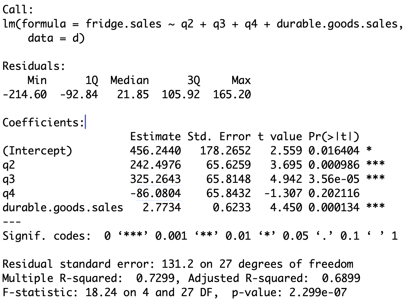
Computing regression coefficients
Call:
lm(formula = fridge.sales ~ q2 + q3 + q4 + durable.goods.sales,
    data = d)
Coefficients:
                    Estimate Std. Error t value Pr(>|t|)
(Intercept)         456.2440   178.2652   2.559 0.016404 *
q2                  242.4976    65.6259   3.695 0.000986 ***
q3                  325.2643    65.8148   4.942 3.56e-05 ***
q4                  -86.0804    65.8432  -1.307 0.202116
durable.goods.sales   2.7734     0.6233   4.450 0.000134 ***
Recall that \, \texttt{Intercept} refers to coefficient for \, \texttt{q1}
Coefficients for \, \texttt{q2}, \texttt{q3}, \texttt{q4} are obtained by summing \, \texttt{Intercept} to coefficient in appropriate row
Computing regression coefficients
Call:
lm(formula = fridge.sales ~ q2 + q3 + q4 + durable.goods.sales,
    data = d)
Coefficients:
                    Estimate Std. Error t value Pr(>|t|)
(Intercept)         456.2440   178.2652   2.559 0.016404 *
q2                  242.4976    65.6259   3.695 0.000986 ***
q3                  325.2643    65.8148   4.942 3.56e-05 ***
q4                  -86.0804    65.8432  -1.307 0.202116
durable.goods.sales 2.7734 0.6233 4.450 0.000134 *** | Variable | Coefficient formula | Estimated coefficient |
|---|---|---|
| \texttt{q1} | \beta_1 | \approx 456.24 |
| \texttt{q2} | \beta_1 + \beta_2 | 456.244 + 242.4976 \approx 698.74 |
| \texttt{q3} | \beta_1 + \beta_3 | 456.244 + 325.2643 \approx 781.51 |
| \texttt{q4} | \beta_1 + \beta_4 | 456.244 - 86.0804 \approx 370.16 |
| D | \beta_5 | \approx 2.77 |
Regression formula and lines
- Therefore, the linear regression formula obtained is
\begin{align*} {\rm I\kern-.3em E}[\text{ Fridge sales } ] = & \,\, 456.24 \times \, \text{Q1} + 698.74 \times \, \text{Q2} + \\[5pts] & \,\, 781.51 \times \, \text{Q3} + 370.16 \times \, \text{Q4} + 2.77 \times \text{D} \end{align*}
- Therefore, we obtain the following regression lines
| Quarter | Regression line |
|---|---|
| Q1 | F = 456.24 + 2.77 \times \text{D} |
| Q2 | F = 698.74 + 2.77 \times \text{D} |
| Q3 | F = 781.51 + 2.77 \times \text{D} |
| Q4 | F = 370.16 + 2.77 \times \text{D} |
- Each quarter has a different intercept: Different baseline fridge sales
Conclusion
- We compare the ANCOVA model to the simple linear model
# Fit simple linear model
linear <- lm(fridge.sales ~ durable.goods.sales, data = d)

# F-test for Model Selection
anova(linear, ancova)
Analysis of Variance Table
Model 1: fridge.sales ~ durable.goods.sales
Model 2: fridge.sales ~ quarter + durable.goods.sales
Res.Df RSS Df Sum of Sq F Pr(>F)
1 30 1377145
2 27 465085 3 912060 17.65 1.523e-06 ***The p-value is p < 0.05 \quad \implies \quad Reject H_0
The ANCOVA model offers a better fit than the linear model