Statistical Models

Lecture 1

Dr. Silvio Fanzon

S.Fanzon@hull.ac.uk

University of Hull

Lecture 1:
An introduction to Statistics

Outline of Lecture 1

1. Module info
2. Introduction
3. Probability revision I
4. Moment generating functions
5. Probability revision II
6. Probability revision III

Part 1:
Module info

Contact details

• Lecturer: Dr. Silvio Fanzon
• Email: S.Fanzon@hull.ac.uk
• Office: Room 104a, Larkin Building
• Office hours: Thursday 15:00-16:00
• Meetings: in my office or send me an Email

Questions

• If you have any questions please feel free to email me

• We will address Homework and Coursework in class

• In addition, please do not hesitate to attend office hours

Lectures

Each week we have

• 2 Lectures of 2h each
• 1 Tutorial of 1h

Session	Date	Place
Lecture 1	Thu 16:00-18:00	Wilberforce LR 4
Lecture 2	Fri 12:00-14:00	Robert Blackburn LTC
Tutorial	Fri 15:00-16:00	Wilberforce LR 3

Assessment

This module will be assessed as follows:

Type of Assessment	Percentage of final grade
Coursework Portfolio	70%
Homework	30%

Rules for Coursework

• Coursework available on Canvas from Week 9

• Coursework must be submitted on Canvas

• Deadline: 14:00 on Thursday 1st May

• No Late Submission allowed

Rules for Homework

• 10 Homework papers, posted weekly on Canvas

• Each Homework paper is worth 14 points

• Final Homework grade computation:

  • Sum the top 7 scores (max score 98 points)
  • Rescale to 100

• Homework must be submitted on Canvas

• Deadline: 14:00 on Thursday

How to submit assignments

• Submit PDFs only on Canvas

• You have two options:

  • Write on tablet and submit PDF Output
  • Write on paper and Scan in Black and White using a Scanner or Scanner App (Tiny Scanner, Scanner Pro, …)

Important: I will not mark

• Assignments submitted outside of Canvas
• Assignments submitted more than 24h After the Deadline

Key submission dates

Assignment	Due date
Homework 1	6 Feb
Homework 2	13 Feb
Homework 3	20 Feb
Homework 4	27 Feb
Homework 5	6 Mar
Homework 6	13 Mar

Assignment	Due date
Homework 7	20 Mar
Homework 8	27 Mar
Homework 9	3 Apr
Homework 10	10 Apr
Easter 😎	14-25 Apr
Coursework	1 May

References

Main textbooks

Slides are self-contained and based on the book

• [1] Bingham, N. H. and Fry, J. M.
  Regression: Linear models in statistics.
  Springer, 2010

References

Main textbooks

.. and also on the book

• [2] Fry, J. M. and Burke, M.
  Quantitative methods in finance using R.
  Open University Press, 2022

References

Secondary References

• [3] Casella, G. and Berger R. L.
  Statistical inference.
  Second Edition, Brooks/Cole, 2002

• [4] DeGroot M. H. and Schervish M. J.
  Probability and Statistics.
  Fourth Edition, Addison-Wesley, 2012

Probability & Statistics manual

Easier Probability & Statistics manual

References

Secondary References

• [5] Dalgaard, P.
  Introductory statistics with R.
  Second Edition, Springer, 2008

• [6] Davies, T. M.
  The book of R.
  No Starch Press, 2016

Concise Statistics with R

Comprehensive R manual

Part 2:
Introduction

The nature of Statistics

• Statistics is a mathematical subject

• We will use a combination of hand calculation and software (R)

• Software (R) is really useful, particularly for dissertations

• Please bring your laptop into class

• Download R onto your laptop

Overview of the module

Module has 11 Lectures, divided into two parts:

• Part I - Mathematical statistics

• Part II - Applied statistics

Overview of the module

Part I - Mathematical statistics

1. Introduction to statistics
2. Normal distribution family and one-sample hypothesis tests
3. Two-sample hypothesis tests
4. The chi-squared test
5. Non-parametric statistics
6. The maths of regression

Overview of the module

Part II - Applied statistics

7. An introduction to practical regression
8. The extra sum of squares principle and regression modelling assumptions
9. Violations of regression assumptions – Autocorrelation
10. Violation of regression assumptions – Multicollinearity
11. ANOVA – Dummy variable regression models

Questions we will address

1. Generic data:

• What is a typical observation
  • What is the mean?
• How spread out is the data?
  • What is the variance?

2. Regression:

• What happens to Y as X increases?
  • increases?
  • decreases?
  • nothing?

Statistics answers these questions systematically

• important for large datasets
• The same mathematical machinery (normal family of distributions) can be applied to both questions

Question 1 – Analysing a general dataset

Two basic questions:

1. Location or mean
2. Spread or variance

Statistics enables to answer systematically:

1. One sample and two-sample t-test
2. Chi-squared test and F-test

Recall the following sketch

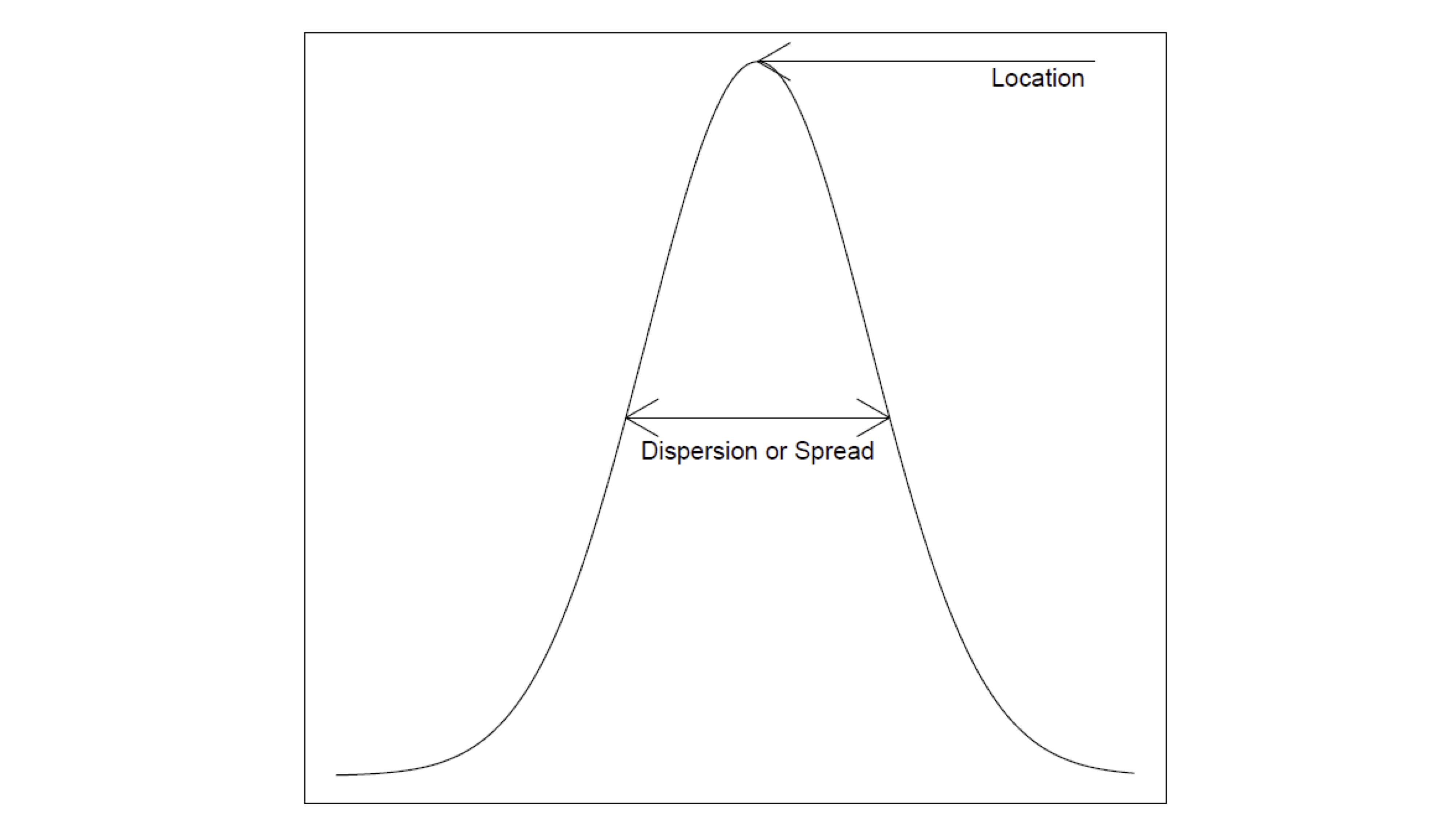
Curve represents data distribution

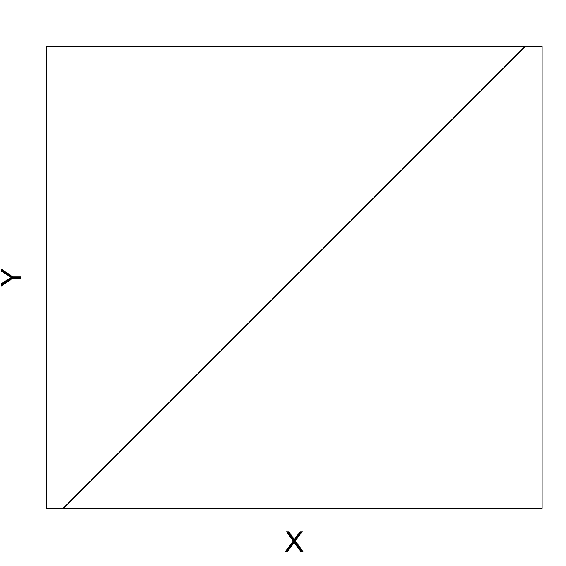
Question 2 – Regression

Basic question in regression:

• What happens to Y as X increases?

  • increases?
  • decreases?
  • nothing?

Regression can be seen as the probabilistic version of (deterministic) linear correlation

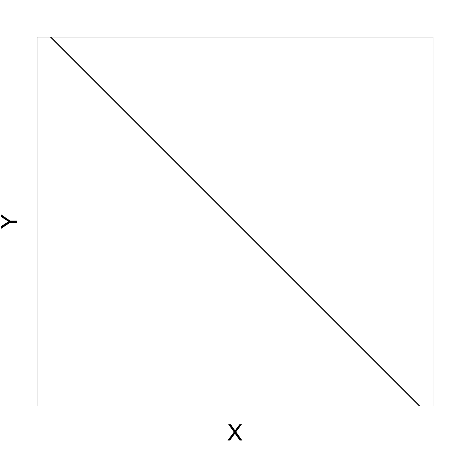
Positive gradient

As X increases Y increases

Negative gradient

As X increases Y decreases

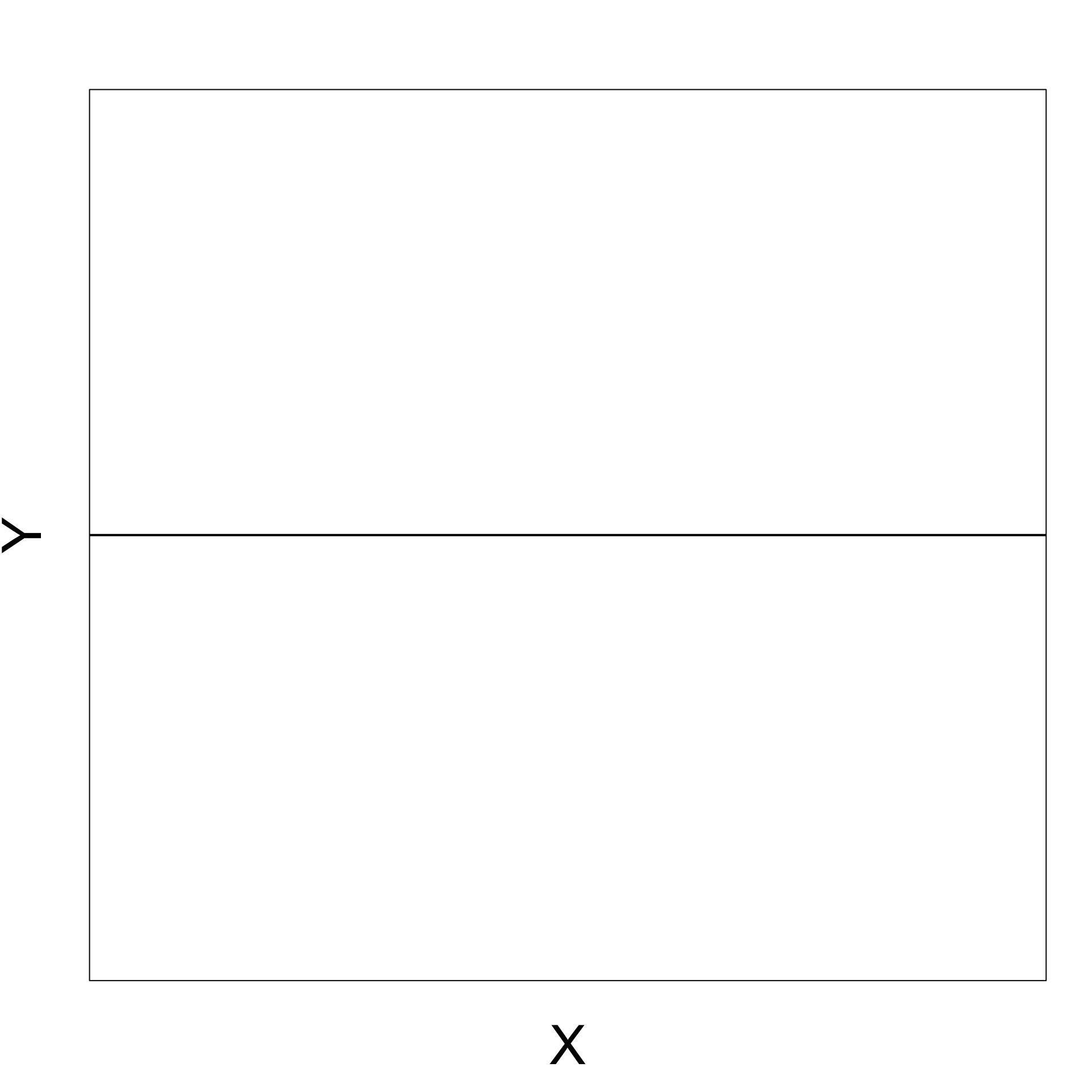
Zero gradient

Changes in X do not affect Y

Real data example

• Real data is more imperfect
• But the same basic idea applies
• Example:
  • X = Stock price
  • Y = Gold price

Real data example

How does real data look like?

Dataset with 33 entries for Stock and Gold price pairs

Stock Price Gold Price 1 3.230426 9.402434 2 2.992937 8.987918 3 2.194025 10.120387 4 2.602475 9.367327 5 2.963497 8.708742 6 4.224242 8.494215 7 7.433981 8.739684 8 5.060836 8.609681 9 3.903316 7.552746 10 4.260542 9.834538 11 3.469490 9.406448

Stock Price Gold Price 12 2.948513 10.62240 13 3.354562 13.12062 14 3.930106 15.05097 15 3.693491 13.39932 16 3.076129 15.34968 17 2.934277 14.83910 18 2.658664 16.01850 19 2.450606 17.25952 20 2.489758 18.26270 21 2.591093 18.13104 22 2.520800 20.20052

Stock Price Gold Price 23 2.471447 24.13767 24 2.062430 30.07695 25 1.805153 35.69485 26 1.673950 39.29658 27 1.620848 39.52317 28 1.547374 36.12564 29 1.721679 31.01106 30 1.974891 29.60810 31 2.168978 35.00593 32 2.277214 37.62929 33 2.993353 41.45828

Real data example

Visualizing the data: Plot Stock Price VS Gold Price

• Observation:
  • As Stock price decreases, Gold price increases
• Why? This might be because:
  • Stock price decreases
  • People invest in secure assets (Gold)
  • Gold demand increases
  • Gold price increases

Real data example

Visualizing the data: Plot Stock Price VS Gold Price

• Inverse proportionality relation evident for dataset

• Question:

  • How likely are we to observe it on new data?

• Regression gives rigorous answer

Part 3:
Probability revision I

Probability revision I

• You are expected to be familiar with the main concepts from Y1 module
  Introduction to Probability & Statistics

• Self-contained revision material available in Appendix A

Topics to review: Sections 1–3 of Appendix A

• Sample space
• Events
• Probability measure
• Conditional probability
• Events independence

• Random Variable (Discrete and Continuous)
• Distribution
• cdf, pmf, pdf
• Expected value and Variance

Summary - Random Variables

• Given probability space (\Omega, \mathcal{B}, P) and a Random Variable X \colon \Omega \to \mathbb{R}

• Cumulative Density Function (cdf): F_X(x) := P(X \leq x)

Discrete RV	Continuous RV
F_X has jumps	F_X is continuous
Probability Mass Function (pmf)	Probability Density Function (pdf)
f_X(x) := P(X=x)	f_X(x) := F_X'(x)
f_X \geq 0	f_X \geq 0
\sum_{x=-\infty}^\infty f_X(x) = 1	\int_{-\infty}^\infty f_X(x) \, dx = 1
F_X (x) = \sum_{k=-\infty}^x f_X(k)	F_X (x) = \int_{-\infty}^x f_X(t) \, dt
P(a \leq X \leq b) = \sum_{k = a}^{b} f_X(k)	P(a \leq X \leq b) = \int_a^b f_X(t) \, dt

Expected Value

• Suppose X \colon \Omega \to \mathbb{R} is RV and g \colon \mathbb{R}\to \mathbb{R} a function
• Then g(X) \colon \Omega \to \mathbb{R} is a RV

Definition

The expected value of the random variable g(X) is

\begin{align*} {\rm I\kern-.3em E}[g(X)] & := \sum_{x} g(x) f_X(x) = \sum_{x \in \mathbb{R}} g(x) P(X = x) \quad \text{ if } X \text{ discrete} \\ {\rm I\kern-.3em E}[g(X)] & := \int_{-\infty}^{\infty} g(x) f_X(x) \, dx \quad \text{ if } X \text{ continuous} \end{align*}

Expected Value

Properties

In particular we have¹

• If X discrete {\rm I\kern-.3em E}[X] = \sum_{x \in \mathbb{R}} x f_X(x) = \sum_{x \in \mathbb{R}} x P(X = x)

• If X continuous {\rm I\kern-.3em E}[X] = \int_{-\infty}^{\infty} x f_X(x) \, dx

1. These follow by taking g(x)=x in previous definitions, so that g(X) = X

Expected Value

Expected value is linear

Theorem

Let X be a rv, and a,b \in \mathbb{R} constants. Then {\rm I\kern-.3em E}[aX + b] = a {\rm I\kern-.3em E}[X] + b

Variance

Variance measures how much a rv X deviates from {\rm I\kern-.3em E}[X]

Definition: Variance

The variance of a random variable X is {\rm Var}[X]:= {\rm I\kern-.3em E}[(X - {\rm I\kern-.3em E}[X])^2]

Proposition: Equivalent formula

{\rm Var}[X] = {\rm I\kern-.3em E}[X^2] - {\rm I\kern-.3em E}[X]^2

Variance

Variance is quadratic

Proposition

X rv and a,b \in \mathbb{R}. Then {\rm Var}[a X + b] = a^2 {\rm Var}[X]

Example - Gamma distribution

Definition

The Gamma distribution with parameters \alpha,\beta>0 is f(x) := \frac{x^{\alpha-1} e^{-\beta{x}} \beta^{\alpha}}{\Gamma(\alpha)} \,, \quad x > 0 where \Gamma is the Gamma function \Gamma(a) :=\int_0^{\infty} x^{a-1} e^{-x} \, dx

Example - Gamma distribution

Definition

Properties of \Gamma:

• The Gamma function coincides with the factorial on natural numbers \Gamma(n)=(n-1)! \,, \quad \forall \, n \in \mathbb{N}

• More in general \Gamma(a)=(a-1)\Gamma(a-1) \,, \quad \forall \, a > 0

• Definition of \Gamma implies normalization of the Gamma distribution: \int_0^{\infty} f(x) \,dx = \int_0^{\infty} \frac{x^{\alpha-1} e^{-\beta{x}} \beta^{\alpha}}{\Gamma(\alpha)} \, dx = 1

Example - Gamma distribution

Definition

X has Gamma distribution with parameters \alpha,\beta if

• the pdf of X is f_X(x) = \begin{cases} \dfrac{x^{\alpha-1} e^{-\beta{x}} \beta^{\alpha}}{\Gamma(\alpha)} & \text{ if } x > 0 \\ 0 & \text{ if } x \leq 0 \end{cases}

• In this case we write X \sim \Gamma(\alpha,\beta)

• \alpha is shape parameter

• \beta is rate parameter

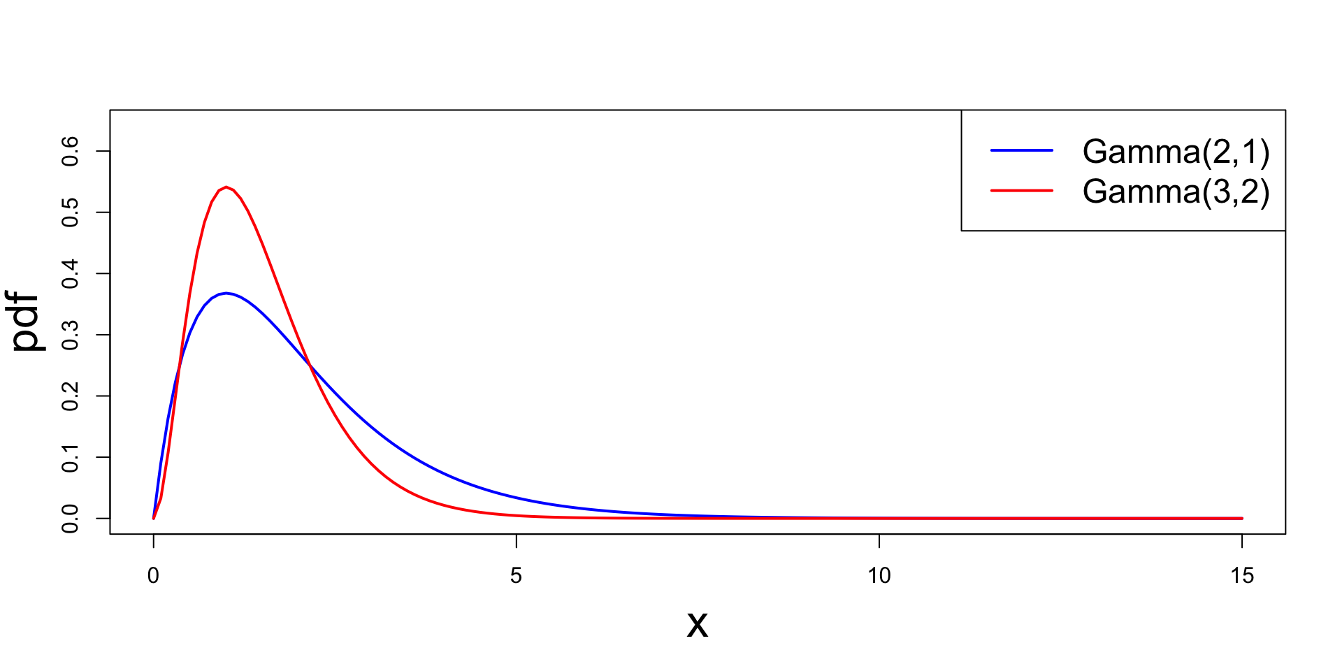
Example - Gamma distribution

Plot

Plotting \Gamma(\alpha,\beta) for parameters (2,1) and (3,2)

Example - Gamma distribution

Expected value

Let X \sim \Gamma(\alpha,\beta). We have: \begin{align*} {\rm I\kern-.3em E}[X] & = \int_{-\infty}^\infty x f_X(x) \, dx \\ & = \int_0^\infty x \, \frac{x^{\alpha-1} e^{-\beta{x}} \beta^{\alpha}}{\Gamma(\alpha)} \, dx \\ & = \frac{ \beta^{\alpha} }{ \Gamma(\alpha) } \int_0^\infty x^{\alpha} e^{-\beta{x}} \, dx \end{align*}

Example - Gamma distribution

Expected value

Recall previous calculation: {\rm I\kern-.3em E}[X] = \frac{ \beta^{\alpha} }{ \Gamma(\alpha) } \int_0^\infty x^{\alpha} e^{-\beta{x}} \, dx Change variable y=\beta x and recall definition of \Gamma: \begin{align*} \int_0^\infty x^{\alpha} e^{-\beta{x}} \, dx & = \int_0^\infty \frac{1}{\beta^{\alpha}} (\beta x)^{\alpha} e^{-\beta{x}} \frac{1}{\beta} \, \beta \, dx \\ & = \frac{1}{\beta^{\alpha+1}} \int_0^\infty y^{\alpha} e^{-y} \, dy \\ & = \frac{1}{\beta^{\alpha+1}} \Gamma(\alpha+1) \end{align*}

Example - Gamma distribution

Expected value

Therefore \begin{align*} {\rm I\kern-.3em E}[X] & = \frac{ \beta^{\alpha} }{ \Gamma(\alpha) } \int_0^\infty x^{\alpha} e^{-\beta{x}} \, dx \\ & = \frac{ \beta^{\alpha} }{ \Gamma(\alpha) } \, \frac{1}{\beta^{\alpha+1}} \Gamma(\alpha+1) \\ & = \frac{\Gamma(\alpha+1)}{\beta \Gamma(\alpha)} \end{align*}

Recalling that \Gamma(\alpha+1)=\alpha \Gamma(\alpha): {\rm I\kern-.3em E}[X] = \frac{\Gamma(\alpha+1)}{\beta \Gamma(\alpha)} = \frac{\alpha}{\beta}

Example - Gamma distribution

Variance

We want to compute {\rm Var}[X] = {\rm I\kern-.3em E}[X^2] - {\rm I\kern-.3em E}[X]^2

• We already have {\rm I\kern-.3em E}[X]
• Need to compute {\rm I\kern-.3em E}[X^2]

Example - Gamma distribution

Variance

Proceeding similarly we have:

\begin{align*} {\rm I\kern-.3em E}[X^2] & = \int_{-\infty}^{\infty} x^2 f_X(x) \, dx \\ & = \int_{0}^{\infty} x^2 \, \frac{ x^{\alpha-1} \beta^{\alpha} e^{- \beta x} }{ \Gamma(\alpha) } \, dx \\ & = \frac{\beta^{\alpha}}{\Gamma(\alpha)} \int_{0}^{\infty} x^{\alpha+1} e^{- \beta x} \, dx \end{align*}

Example - Gamma distribution

Variance

Recall previous calculation: {\rm I\kern-.3em E}[X^2] = \frac{\beta^{\alpha}}{\Gamma(\alpha)} \int_{0}^{\infty} x^{\alpha+1} e^{- \beta x} \, dx Change variable y=\beta x and recall definition of \Gamma: \begin{align*} \int_0^\infty x^{\alpha+1} e^{-\beta{x}} \, dx & = \int_0^\infty \frac{1}{\beta^{\alpha+1}} (\beta x)^{\alpha + 1} e^{-\beta{x}} \frac{1}{\beta} \, \beta \, dx \\ & = \frac{1}{\beta^{\alpha+2}} \int_0^\infty y^{\alpha + 1 } e^{-y} \, dy \\ & = \frac{1}{\beta^{\alpha+2}} \Gamma(\alpha+2) \end{align*}

Example - Gamma distribution

Variance

Therefore {\rm I\kern-.3em E}[X^2] = \frac{ \beta^{\alpha} }{ \Gamma(\alpha) } \int_0^\infty x^{\alpha+1} e^{-\beta{x}} \, dx = \frac{ \beta^{\alpha} }{ \Gamma(\alpha) } \, \frac{1}{\beta^{\alpha+2}} \Gamma(\alpha+2) = \frac{\Gamma(\alpha+2)}{\beta^2 \Gamma(\alpha)} Now use following formula twice \Gamma(\alpha+1)=\alpha \Gamma(\alpha): \Gamma(\alpha+2)= (\alpha + 1) \Gamma(\alpha + 1) = (\alpha + 1) \alpha \Gamma(\alpha) Substituting we get {\rm I\kern-.3em E}[X^2] = \frac{\Gamma(\alpha+2)}{\beta^2 \Gamma(\alpha)} = \frac{(\alpha+1) \alpha}{\beta^2}

Example - Gamma distribution

Variance

Therefore {\rm I\kern-.3em E}[X] = \frac{\alpha}{\beta} \quad \qquad {\rm I\kern-.3em E}[X^2] = \frac{(\alpha+1) \alpha}{\beta^2} and the variance is \begin{align*} {\rm Var}[X] & = {\rm I\kern-.3em E}[X^2] - {\rm I\kern-.3em E}[X]^2 \\ & = \frac{(\alpha+1) \alpha}{\beta^2} - \frac{\alpha^2}{\beta^2} \\ & = \frac{\alpha}{\beta^2} \end{align*}

Part 4:
Moment generating functions

Moment generating function

• We abbreviate Moment generating function with MGF

• MGF provides a short-cut to calculating mean and variance

Definition

The moment generating function or MGF of a rv X is M_X(t) := {\rm I\kern-.3em E}[e^{tX}] \,, \quad \forall \, t \in \mathbb{R}

In particular we have:

• X discrete: M_X(t) = \sum_{x \in \mathbb{R}} e^{tx} f_X(x)

• X continuous: M_X(t) = \int_{-\infty}^\infty e^{tx} f_X(x) \, dx

Moment generating function

Computing moments

Theorem

If X has MGF M_X then {\rm I\kern-.3em E}[X^n] = M_X^{(n)} (0) where we denote M_X^{(n)} (0) := \frac{d^n}{dt^n} M_X^{(n)}(t) \bigg|_{t=0}

The quantity {\rm I\kern-.3em E}[X^n] is called n-th moment of X

Moment generating function

Proof of Theorem

Suppose X continuous and that we can exchange derivative and integral: \begin{align*} \frac{d}{dt} M_X(t) & = \frac{d}{dt} \int_{-\infty}^\infty e^{tx} f_X(x) \, dx = \int_{-\infty}^\infty \left( \frac{d}{dt} e^{tx} \right) f_X(x) \, dx \\ & = \int_{-\infty}^\infty xe^{tx} f_X(x) \, dx = {\rm I\kern-.3em E}(Xe^{tX}) \end{align*} Evaluating at t = 0: \frac{d}{dt} M_X(t) \bigg|_{t = 0} = {\rm I\kern-.3em E}(Xe^{0}) = {\rm I\kern-.3em E}[X]

Moment generating function

Proof of Theorem

Proceeding by induction we obtain: \frac{d^n}{dt^n} M_X(t) = {\rm I\kern-.3em E}(X^n e^{tX}) Evaluating at t = 0 yields the thesis: \frac{d^n}{dt^n} M_X(t) \bigg|_{t = 0} = {\rm I\kern-.3em E}(X^n e^{0}) = {\rm I\kern-.3em E}[X^n]

Moment generating function

Notation

For the first 3 derivatives we use special notations:

M_X'(0) := M^{(1)}_X(0) = {\rm I\kern-.3em E}[X] M_X''(0) := M^{(2)}_X(0) = {\rm I\kern-.3em E}[X^2] M_X'''(0) := M^{(3)}_X(0) = {\rm I\kern-.3em E}[X^3]

Example - Normal distribution

Definition

• The normal distribution with mean \mu and variance \sigma^2 is f(x) := \frac{1}{\sqrt{2\pi\sigma^2}} \, \exp\left( -\frac{(x-\mu)^2}{2\sigma^2}\right) \,, \quad x \in \mathbb{R}

• X has normal distribution with mean \mu and variance \sigma^2 if f_X = f

  • In this case we write X \sim N(\mu,\sigma^2)

• The standard normal distribution is denoted N(0,1)

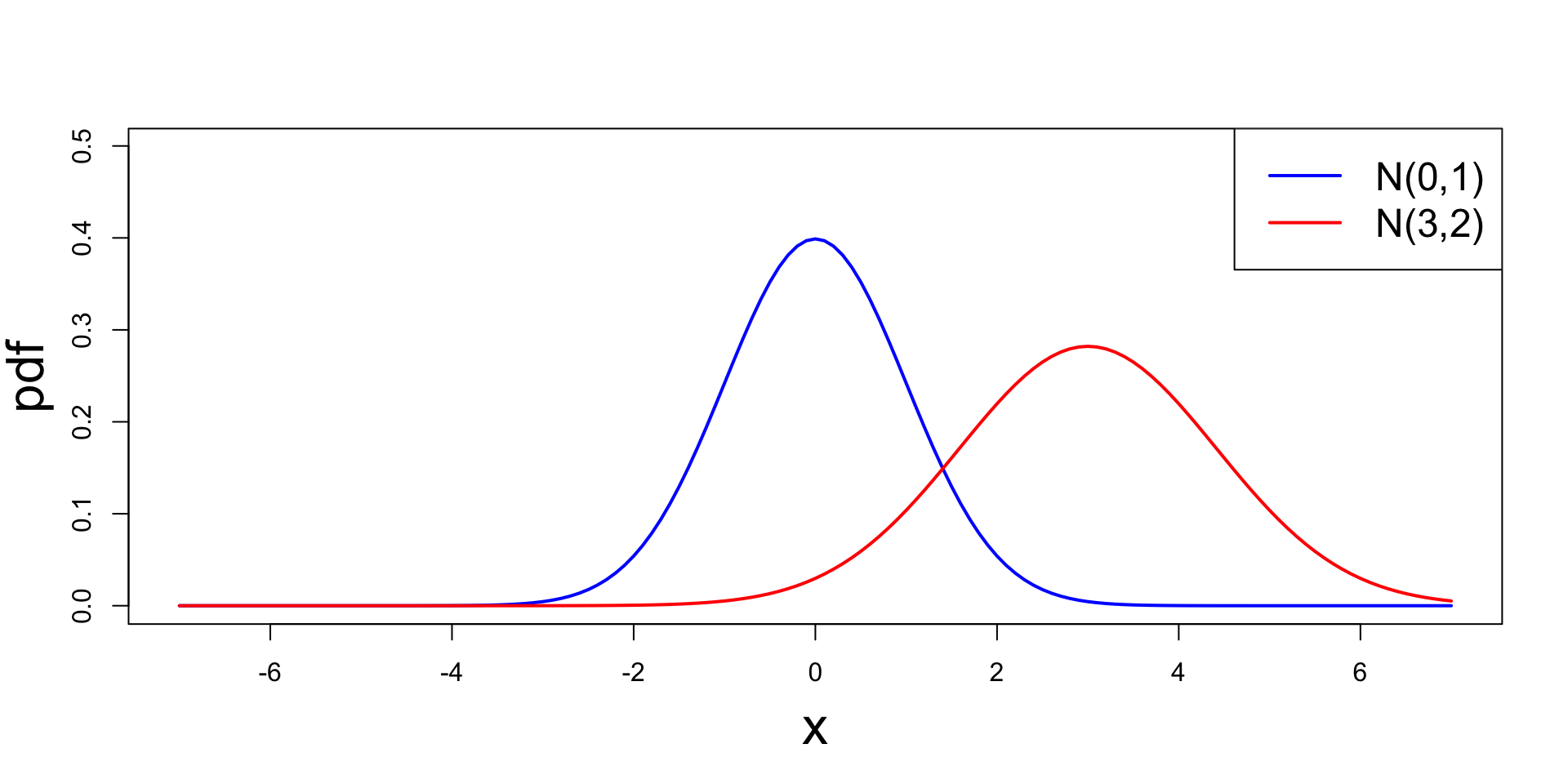
Example - Normal distribution

Plot

Plotting N(\mu,\sigma^2) for parameters (0,1) and (3,2)

Example - Normal distribution

Moment generating function

The equation for the normal pdf is f_X(x) = \frac{1}{\sqrt{2\pi\sigma^2}} \, \exp\left(-\frac{(x-\mu)^2}{2\sigma^2}\right) Being pdf, we must have \int f_X(x) \, dx = 1. This yields: \begin{equation} \tag{1} \int_{-\infty}^{\infty} \exp \left( -\frac{x^2}{2\sigma^2} + \frac{\mu{x}}{\sigma^2} \right) \, dx = \exp \left(\frac{\mu^2}{2\sigma^2} \right) \sqrt{2\pi} \sigma \end{equation}

Example - Normal distribution

Moment generating function

We have \begin{align*} M_X(t) & := {\rm I\kern-.3em E}(e^{tX}) = \int_{-\infty}^{\infty} e^{tx} f_X(x) \, dx \\ & = \int_{-\infty}^{\infty} e^{tx} \frac{1}{\sqrt{2\pi}\sigma} \exp \left( -\frac{(x-\mu)^2}{2\sigma^2} \right) \, dx \\ & = \frac{1}{\sqrt{2\pi}\sigma} \int_{-\infty}^{\infty} e^{tx} \exp \left( -\frac{x^2}{2\sigma^2} - \frac{\mu^2}{2\sigma^2} + \frac{x\mu}{\sigma^2} \right) \, dx \\ & = \exp\left(-\frac{\mu^2}{2\sigma^2} \right) \frac{1}{\sqrt{2\pi}\sigma} \int_{-\infty}^{\infty} \exp \left(- \frac{x^2}{2\sigma^2} + \frac{(t\sigma^2+\mu) x}{\sigma^2} \right) \, dx \end{align*}

Example - Normal distribution

Moment generating function

We have shown \begin{equation} \tag{2} M_X(t) = \exp\left(-\frac{\mu^2}{2\sigma^2} \right) \frac{1}{\sqrt{2\pi}\sigma} \int_{-\infty}^{\infty} \exp \left(- \frac{x^2}{2\sigma^2} + \frac{(t\sigma^2+\mu) x}{\sigma^2} \right) \, dx \end{equation} Replacing \mu by (t\sigma^2 + \mu) in (1) we obtain \begin{equation} \tag{3} \int_{-\infty}^{\infty} \exp \left(- \frac{x^2}{2\sigma^2} + \frac{(t\sigma^2+\mu) x}{\sigma^2} \right) \, dx = \exp \left( \frac{(t\sigma^2+\mu)^2}{2\sigma^2} \right) \, \sqrt{2\pi}\sigma \end{equation} Substituting (3) in (2) and simplifying we get M_X(t) = \exp \left( \mu t + \frac{t^2 \sigma^2}{2} \right)

Example - Normal distribution

Mean

Recall the mgf M_X(t) = \exp \left( \mu t + \frac{t^2 \sigma^2}{2} \right) The first derivative is M_X'(t) = (\mu + \sigma^2 t ) \exp \left( \mu t + \frac{t^2 \sigma^2}{2} \right) Therefore the mean: {\rm I\kern-.3em E}[X] = M_X'(0) = \mu

Example - Normal distribution

Variance

The first derivative of mgf is M_X'(t) = (\mu + \sigma^2 t ) \exp \left( \mu t + \frac{t^2 \sigma^2}{2} \right) The second derivative is then M_X''(t) = \sigma^2 \exp \left( \mu t + \frac{t^2 \sigma^2}{2} \right) + (\mu + \sigma^2 t )^2 \exp \left( \mu t + \frac{t^2 \sigma^2}{2} \right) Therefore the second moment is: {\rm I\kern-.3em E}[X^2] = M_X''(0) = \sigma^2 + \mu^2

Example - Normal distribution

Variance

We have seen that: {\rm I\kern-.3em E}[X] = \mu \quad \qquad {\rm I\kern-.3em E}[X^2] = \sigma^2 + \mu^2 Therefore the variance is: \begin{align*} {\rm Var}[X] & = {\rm I\kern-.3em E}[X^2] - {\rm I\kern-.3em E}[X]^2 \\ & = \sigma^2 + \mu^2 - \mu^2 \\ & = \sigma^2 \end{align*}

Example - Gamma distribution

Moment generating function

Suppose X \sim \Gamma(\alpha,\beta). This means f_X(x) = \begin{cases} \dfrac{x^{\alpha-1} e^{-\beta{x}} \beta^{\alpha}}{\Gamma(\alpha)} & \text{ if } x > 0 \\ 0 & \text{ if } x \leq 0 \end{cases}

• We have seen already that {\rm I\kern-.3em E}[X] = \frac{\alpha}{\beta} \quad \qquad {\rm Var}[X] = \frac{\alpha}{\beta^2}

• We want to compute mgf M_X to derive again {\rm I\kern-.3em E}[X] and {\rm Var}[X]

Example - Gamma distribution

Moment generating function

We compute \begin{align*} M_X(t) & = {\rm I\kern-.3em E}[e^{tX}] = \int_{-\infty}^\infty e^{tx} f_X(x) \, dx \\ & = \int_0^{\infty} e^{tx} \, \frac{x^{\alpha-1}e^{-\beta{x}} \beta^{\alpha}}{\Gamma(\alpha)} \, dx \\ & = \frac{\beta^{\alpha}}{\Gamma(\alpha)}\int_0^{\infty}x^{\alpha-1}e^{-(\beta-t)x} \, dx \end{align*}

Example - Gamma distribution

Moment generating function

From the previous slide we have M_X(t) = \frac{\beta^{\alpha}}{\Gamma(\alpha)}\int_0^{\infty}x^{\alpha-1}e^{-(\beta-t)x} \, dx Change variable y=(\beta-t)x and recall the definition of \Gamma: \begin{align*} \int_0^{\infty} x^{\alpha-1} e^{-(\beta-t)x} \, dx & = \int_0^{\infty} \frac{1}{(\beta-t)^{\alpha-1}} [(\beta-t)x]^{\alpha-1} e^{-(\beta-t)x} \frac{1}{(\beta-t)} (\beta - t) \, dx \\ & = \frac{1}{(\beta-t)^{\alpha}} \int_0^{\infty} y^{\alpha-1} e^{-y} \, dy \\ & = \frac{1}{(\beta-t)^{\alpha}} \Gamma(\alpha) \end{align*}

Example - Gamma distribution

Moment generating function

Therefore \begin{align*} M_X(t) & = \frac{\beta^{\alpha}}{\Gamma(\alpha)}\int_0^{\infty}x^{\alpha-1}e^{-(\beta-t)x} \, dx \\ & = \frac{\beta^{\alpha}}{\Gamma(\alpha)} \cdot \frac{1}{(\beta-t)^{\alpha}} \Gamma(\alpha) \\ & = \frac{\beta^{\alpha}}{(\beta-t)^{\alpha}} \end{align*}

Example - Gamma distribution

Expectation

From the mgf M_X(t) = \frac{\beta^{\alpha}}{(\beta-t)^{\alpha}} we compute the first derivative: \begin{align*} M_X'(t) & = \frac{d}{dt} [\beta^{\alpha}(\beta-t)^{-\alpha}] \\ & = \beta^{\alpha}(-\alpha)(\beta-t)^{-\alpha-1}(-1) \\ & = \alpha\beta^{\alpha}(\beta-t)^{-\alpha-1} \end{align*}

Example - Gamma distribution

Expectation

From the first derivative M_X'(t) = \alpha\beta^{\alpha}(\beta-t)^{-\alpha-1} we compute the expectation \begin{align*} {\rm I\kern-.3em E}[X] & = M_X'(0) \\ & = \alpha\beta^{\alpha}(\beta)^{-\alpha-1} \\ & =\frac{\alpha}{\beta} \end{align*}

Example - Gamma distribution

Variance

From the first derivative M_X'(t) = \alpha\beta^{\alpha}(\beta-t)^{-\alpha-1} we compute the second derivative \begin{align*} M_X''(t) & = \frac{d}{dt}[\alpha\beta^{\alpha}(\beta-t)^{-\alpha-1}] \\ & = \alpha\beta^{\alpha}(-\alpha-1)(\beta-t)^{-\alpha-2}(-1)\\ & = \alpha(\alpha+1)\beta^{\alpha}(\beta-t)^{-\alpha-2} \end{align*}

Example - Gamma distribution

Variance

From the second derivative M_X''(t) = \alpha(\alpha+1)\beta^{\alpha}(\beta-t)^{-\alpha-2} we compute the second moment: \begin{align*} {\rm I\kern-.3em E}[X^2] & = M_X''(0) \\ & = \alpha(\alpha+1)\beta^{\alpha}(\beta)^{-\alpha-2} \\ & = \frac{\alpha(\alpha + 1)}{\beta^2} \end{align*}

Example - Gamma distribution

Variance

From the first and second moments: {\rm I\kern-.3em E}[X] = \frac{\alpha}{\beta} \qquad \qquad {\rm I\kern-.3em E}[X^2] = \frac{\alpha(\alpha + 1)}{\beta^2} we can compute the variance \begin{align*} {\rm Var}[X] & = {\rm I\kern-.3em E}[X^2] - {\rm I\kern-.3em E}[X]^2 \\ & = \frac{\alpha(\alpha + 1)}{\beta^2} - \frac{\alpha^2}{\beta^2} \\ & = \frac{\alpha}{\beta^2} \end{align*}

Moment generating function

The mgf characterizes a distribution

Theorem

Let X and Y be random variables with mgfs M_X and M_Y respectively. Assume there exists \varepsilon>0 such that M_X(t) = M_Y(t) \,, \quad \forall \, t \in (-\varepsilon, \varepsilon) Then X and Y have the same cdf F_X(u) = F_Y(u) \,, \quad \forall \, x \in \mathbb{R}

In other words: \qquad same mgf \quad \implies \quad same distribution

Example

• Suppose X is a random variable such that M_X(t) = \exp \left( \mu t + \frac{t^2 \sigma^2}{2} \right) As the above is the mgf of a normal distribution, by the previous Theorem we infer X \sim N(\mu,\sigma^2)

• Suppose Y is a random variable such that M_Y(t) = \frac{\beta^{\alpha}}{(\beta-t)^{\alpha}} As the above is the mgf of a Gamma distribution, by the previous Theorem we infer Y \sim \Gamma(\alpha,\beta)

Part 5:
Probability revision II

Probability revision II

• You are expected to be familiar with the main concepts from Y1 module
  Introduction to Probability & Statistics

• Self-contained revision material available in Appendix A

Topics to review: Sections 4–5 of Appendix A

• Random vectors
• Bivariate vectors
• Joint pdf and pmf
• Marginals

• Conditional distributions
• Conditional expectation
• Conditional variance

Univariate vs Bivariate vs Multivariate

• Probability models seen so far only involve 1 random variable
  • These are called univariate models
• We are also interested in probability models involving multiple variables:
  • Models with 2 random variables are called bivariate
  • Models with more than 2 random variables are called multivariate

Random vectors

Definition

Recall: a random variable is a measurable function X \colon \Omega \to \mathbb{R}\,, \quad \Omega \,\, \text{ sample space}

Definition

A random vector is a measurable function \mathbf{X}\colon \Omega \to \mathbb{R}^n. We say that

• \mathbf{X} is univariate if n=1
• \mathbf{X} is bivariate if n=2
• \mathbf{X} is multivariate if n \geq 3

Random vectors

Notation

• The components of a random vector \mathbf{X} are denoted by \mathbf{X}= (X_1, \ldots, X_n) with X_i \colon \Omega \to \mathbb{R} random variables

• We denote a two-dimensional bivariate random vector by (X,Y) with X,Y \colon \Omega \to \mathbb{R} random variables

Summary - Bivariate Random Vectors

(X,Y) discrete random vector	(X,Y) continuous random vector
X and Y discrete RV	X and Y continuous RV
Joint pmf	Joint pdf
f_{X,Y}(x,y) := P(X=x,Y=y)	P((X,Y) \in A) = \int_A f_X(x,y) \,dxdy
f_{X,Y} \geq 0	f_{X,Y} \geq 0
\sum_{(x,y)\in \mathbb{R}^2} f_{X,Y}(x,y)=1	\int_{\mathbb{R}^2} f_{X,Y}(x,y) \, dxdy= 1
Marginal pmfs	Marginal pdfs
f_X (x) := P(X=x)	P(a \leq X \leq b) = \int_a^b f_X(x) \,dx
f_Y (y) := P(Y=y)	P(a \leq Y \leq b) = \int_a^b f_Y(y) \,dy
f_X (x)=\sum_{y \in \mathbb{R}} f_{X,Y}(x,y)	f_X(x) = \int_{\mathbb{R}} f_{X,Y}(x,y) \,dy
f_Y (y)=\sum_{x \in \mathbb{R}} f_{X,Y}(x,y)	f_Y(y) = \int_{\mathbb{R}} f_{X,Y}(x,y) \,dx

Expected Value

• Suppose (X,Y) \colon \Omega \to \mathbb{R}^2 is random vector and g \colon \mathbb{R}^2 \to \mathbb{R} function
• Then g(X,Y) \colon \Omega \to \mathbb{R} is random variable

Definition

The expected value of the random variable g(X,Y) is \begin{align*} {\rm I\kern-.3em E}[g(X,Y)] & := \sum_{x,y} g(x,y) P(X=x,Y=y) \quad \text{ if } (X,Y) \text{ discrete} \\ {\rm I\kern-.3em E}[g(X,Y)] & := \int_{\mathbb{R}^2} g(x,y) f_{X,Y}(x,y) \, dxdy \quad \text{ if } (X,Y) \text{ continuous} \end{align*}

Notation:The symbol \int_{\mathbb{R}^2} denotes the double integral \int_{-\infty}^\infty\int_{-\infty}^\infty

Conditional distributions

(X,Y) rv with joint pdf (or pmf) f_{X,Y} and marginal pdfs (or pmfs) f_X, f_Y

• The conditional pdf (or pmf) of Y given that X=x is the function f(\cdot | x) f(y|x) := \frac{f_{X,Y}(x,y)}{f_X(x)} \, , \qquad \text{ whenever} \quad f_X(x)>0

• The conditional pdf (or pmf) of X given that Y=y is the function f(\cdot | y) f(x|y) := \frac{f_{X,Y}(x,y)}{f_Y(y)}\, , \qquad \text{ whenever} \quad f_Y(y)>0

• Notation: We will often write

  • Y|X to denote the distribution f(y|x)
  • X|Y to denote the distribution f(x|y)

Conditional expectation

Definition

(X,Y) random vector and g \colon \mathbb{R}\to \mathbb{R} function. The conditional expectation of g(Y) given X=x is \begin{align*} {\rm I\kern-.3em E}[g(Y) | x] & := \sum_{y} g(y) f(y|x) \quad \text{ if } (X,Y) \text{ discrete} \\ {\rm I\kern-.3em E}[g(Y) | x] & := \int_{y \in \mathbb{R}} g(y) f(y|x) \, dy \quad \text{ if } (X,Y) \text{ continuous} \end{align*}

• {\rm I\kern-.3em E}[g(Y) | x] is a real number for all x \in \mathbb{R}
• {\rm I\kern-.3em E}[g(Y) | X] denotes the Random Variable h(X) where h(x):={\rm I\kern-.3em E}[g(Y) | x]

Conditional variance

Definition

(X,Y) random vector. The conditional variance of Y given X=x is {\rm Var}[Y | x] := {\rm I\kern-.3em E}[Y^2|x] - {\rm I\kern-.3em E}[Y|x]^2

• {\rm Var}[Y | x] is a real number for all x \in \mathbb{R}
• {\rm Var}[Y | X] denotes the Random Variable {\rm Var}[Y | X] := {\rm I\kern-.3em E}[Y^2|X] - {\rm I\kern-.3em E}[Y|X]^2

Exercise - Conditional distribution

Assume given a continuous random vector (X,Y) with joint pdf f_{X,Y}(x,y) := e^{-y} \,\, \text{ if } \,\, 0 < x < y \,, \quad f_{X,Y}(x,y) :=0 \,\, \text{ otherwise}

• Compute f_X and f(y|x)
• Compute {\rm I\kern-.3em E}[Y|X]
• Compute {\rm Var}[Y|X]

Solution

• We compute f_X, the marginal pdf of X:
  • If x \leq 0 then f_{X,Y}(x,y)=0. Therefore f_X(x) = \int_{-\infty}^\infty f_{X,Y}(x,y) \, dy = 0
  • If x > 0 then f_{X,Y}(x,y)=e^{-y} if y>x, and f_{X,Y}(x,y)=0 if y \leq x. Thus \begin{align*} f_X(x) & = \int_{-\infty}^\infty f_{X,Y}(x,y) \, dy = \int_{x}^\infty e^{-y} \, dy \\ & = - e^{-y} \bigg|_{y=x}^{y=\infty} = -e^{-\infty} + e^{-x} = e^{-x} \end{align*}

Solution

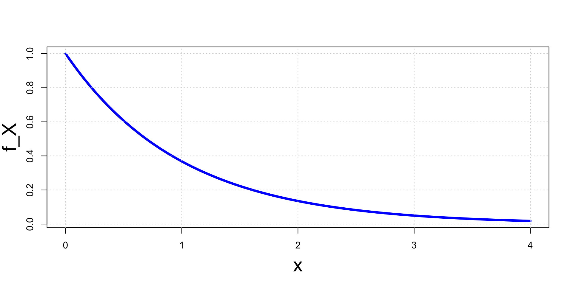
• The marginal pdf of X has then exponential distribution f_{X}(x) = \begin{cases} e^{-x} & \text{ if } x > 0 \\ 0 & \text{ if } x \leq 0 \end{cases}

Solution

• We now compute f(y|x), the conditional pdf of Y given X=x:
  • Note that f_X(x)>0 for all x>0
  • Hence assume fixed some x>0
  • If y>x we have f_{X,Y}(x,y)=e^{-y}. Hence f(y|x) := \frac{f_{X,Y}(x,y)}{f_X(x)} = \frac{e^{-y}}{e^{-x}} = e^{-(y-x)}
  • If y \leq x we have f_{X,Y}(x,y)=0. Hence f(y|x) := \frac{f_{X,Y}(x,y)}{f_X(x)} = \frac{0}{e^{-x}} = 0

Solution

• The conditional distribution Y|X is therefore exponential, shifted by x f(y|x) = \begin{cases} e^{-(y-x)} & \text{ if } y > x \\ 0 & \text{ if } y \leq x \end{cases}

• The conditional expectation of Y given X=x is \begin{align*} {\rm I\kern-.3em E}[Y|x] & = \int_{-\infty}^\infty y f(y|x) \, dy = \int_{x}^\infty y e^{-(y-x)} \, dy \\ & = -(y+1) e^{-(y-x)} \bigg|_{x}^\infty = x + 1 \end{align*} where we integrated by parts

Solution

• Therefore conditional expectation of Y given X=x is {\rm I\kern-.3em E}[Y|x] = x + 1

• This can also be interpreted as the random variable {\rm I\kern-.3em E}[Y|X] = X + 1

• This is not surprising!

  • The distribution of Y|X is just an exponential translated by X
  • Therefore, the expected value of Y|X is the expected value of the exponential distribution, which is 1, translated by X

Solution

• The conditional second moment of Y given X=x is \begin{align*} {\rm I\kern-.3em E}[Y^2|x] & = \int_{-\infty}^\infty y^2 f(y|x) \, dy = \int_{x}^\infty y^2 e^{-(y-x)} \, dy \\ & = (y^2+2y+2) e^{-(y-x)} \bigg|_{x}^\infty = x^2 + 2x + 2 \end{align*} where we integrated by parts

• The conditional variance of Y given X=x is {\rm Var}[Y|x] = {\rm I\kern-.3em E}[Y^2|x] - {\rm I\kern-.3em E}[Y|x]^2 = x^2 + 2x + 2 - (x+1)^2 = 1

Solution

• The conditional variance can be interpreted as the random variable {\rm Var}[Y|X] = 1

• This is not surprising!

  • The distribution of Y|X is just an exponential translated by X
  • Therefore, the shape of the distribution does not change
  • Thus, the variance of Y|X does not depend on X {\rm Var}[Y|X = x ] = {\rm Var}[Y | X = 0] = 1

Conditional Expectation

A useful formula

Theorem

(X,Y) random vector. Then {\rm I\kern-.3em E}[X] = {\rm I\kern-.3em E}[ {\rm I\kern-.3em E}[X|Y] ]

Note: The above formula contains abuse of notation – {\rm I\kern-.3em E} has 3 meanings

• First {\rm I\kern-.3em E} is with respect to the marginal of X
• Second {\rm I\kern-.3em E} is with respect to the marginal of Y
• Third {\rm I\kern-.3em E} is with respect to the conditional distribution X|Y

Conditional Variance

A useful formula

Theorem

(X,Y) random vector. Then {\rm Var}[X] = {\rm I\kern-.3em E}[ {\rm Var}[ X|Y] ] + {\rm Var}[{\rm I\kern-.3em E}[X|Y]]

Exercise

Let n \in \mathbb{N} be constant, and the random vector (X,Y) satisfy the following:

• X has uniform distribution on [0,1], meaning that its pdf is f_X(x) = \chi_{[0,1]}(x) = \begin{cases} 1 & \, \text{ if } \, x \in [0,1] \\ 0 & \, \text{ otherwise } \end{cases}

• The distribution of Y, conditional on X = x, is binomial \mathop{\mathrm{Bin}}(n,x). This means P(Y = k | X = x) = \binom{n}{k} x^k (1-x)^{n-k} \,, \quad k = 0 , 1 , \ldots ,n \,, where the binomial coefficient is \binom{n}{k} = \frac{n!}{k!(n-k)!}

Question: Compute {\rm I\kern-.3em E}[Y] and {\rm Var}[Y]

Solution

• By assumption X is uniform on [0,1]. Therefore \begin{align*} f_X(x) & = \chi_{[0,1]}(x) = \begin{cases} 1 & \, \text{ if } \, x \in [0,1] \\ 0 & \, \text{ otherwise } \end{cases} \\ {\rm I\kern-.3em E}[X] & = \int_\mathbb{R}x f_{X}(x)\, dx = \int_0^1 x \, dx = \frac12 \\ {\rm I\kern-.3em E}[X^2] & = \int_\mathbb{R}x^2 f_{X} (x)\, dx = \int_0^1 x^2 \, dx = \frac13 \\ {\rm Var}[X] & = {\rm I\kern-.3em E}[X^2] - {\rm I\kern-.3em E}[X]^2 = \frac13 - \frac{1}{4} = \frac{1}{12} \end{align*}

Solution

• By assumption Y | X = x is \mathop{\mathrm{Bin}}(n,x). Using well-known formulas, we get {\rm I\kern-.3em E}[Y|X] = nX \,, \qquad {\rm Var}[Y|X] = nX(1-X)

• Therefore we conclude \begin{align*} {\rm I\kern-.3em E}[Y] & = {\rm I\kern-.3em E}[ {\rm I\kern-.3em E}[Y|X] ] = {\rm I\kern-.3em E}[nX] = n {\rm I\kern-.3em E}[X] = \frac{n}{2} \\ & \phantom{s} \\ {\rm Var}[Y] & = {\rm I\kern-.3em E}[{\rm Var}[Y|X]] + {\rm Var}[{\rm I\kern-.3em E}[Y|X]] \\ & = {\rm I\kern-.3em E}[nX(1-X)] + {\rm Var}[nX] \\ & = n {\rm I\kern-.3em E}[X] - n{\rm I\kern-.3em E}[X^2] + n^2{\rm Var}[X] \\ & = \frac{n}{2} - \frac{n}{3} + \frac{n^2}{12} = \frac{n}{6} + \frac{n^2}{12} \end{align*}

Part 6:
Probability revision III

Probability revision III

• You are expected to be familiar with the main concepts from Y1 module
  Introduction to Probability & Statistics

• Self-contained revision material available in Appendix A

Topics to review: Sections 6–7 of Appendix A

• Independence of random variables
• Covariance and correlation

Independence of random variables

Definition: Independence

(X,Y) random vector with joint pdf or pmf f_{X,Y} and marginal pdfs or pmfs f_X,f_Y. We say that X and Y are independent random variables if f_{X,Y}(x,y) = f_X(x)f_Y(y) \,, \quad \forall \, (x,y) \in \mathbb{R}^2

Independence of random variables

Conditional distributions and probabilities

If X and Y are independent then X gives no information on Y (and vice-versa):

• Conditional distribution: Y|X is same as Y f(y|x) = \frac{f_{X,Y}(x,y)}{f_X(x)} = \frac{f_X(x)f_Y(y)}{f_X(x)} = f_Y(y)

• Conditional probabilities: From the above we also obtain \begin{align*} P(Y \in A | x) & = \sum_{y \in A} f(y|x) = \sum_{y \in A} f_Y(y) = P(Y \in A) & \, \text{ discrete rv} \\ P(Y \in A | x) & = \int_{y \in A} f(y|x) \, dy = \int_{y \in A} f_Y(y) \, dy = P(Y \in A) & \, \text{ continuous rv} \end{align*}

Independence of random variables

Characterization of independence - Densities

Theorem

(X,Y) random vector with joint pdf or pmf f_{X,Y}. They are equivalent:

• X and Y are independent random variables
• There exist functions g(x) and h(y) such that f_{X,Y}(x,y) = g(x)h(y) \,, \quad \forall \, (x,y) \in \mathbb{R}^2

Note:

• g(x) and h(y) are not necessarily the pdfs or pmfs of X and Y
• However they coincide with f_X and f_Y, up to rescaling by a constant

Exercise

A student leaves for class between 8 AM and 8:30 AM and takes between 40 and 50 minutes to get there

• Denote by X the time of departure

  • X = 0 corresponds to 8 AM
  • X = 30 corresponds to 8:30 AM

• Denote by Y the travel time

• Assume that X and Y are independent and uniformly distributed

Question: Find the probability that the student arrives to class before 9 AM

Solution

• By assumption X is uniform on (0,30). Therefore f_X(x) = \begin{cases} \frac{1}{30} & \text{ if } \, x \in (0,30) \\ 0 & \text{ otherwise } \end{cases}

• By assumption Y is uniform on (40,50). Therefore f_Y(y) = \begin{cases} \frac{1}{10} & \text{ if } \, y \in (40,50) \\ 0 & \text{ otherwise } \end{cases} where we used that 50 - 40 = 10

Solution

• Define the rectangle R = (0,30) \times (40,50)

• Since X and Y are independent, we get

f_{X,Y}(x,y) = f_X(x)f_Y(y) = \begin{cases} \frac{1}{300} & \text{ if } \, (x,y) \in R \\ 0 & \text{ otherwise } \end{cases}

Solution

• The arrival time is given by X + Y

• Therefore, the student arrives to class before 9 AM iff X + Y < 60

• Notice that \{X + Y < 60 \} = \{ (x,y) \in \mathbb{R}^2 \, \colon \, 0 \leq x < 60 - y, 40 \leq y < 50 \}

Solution

Therefore, the probability of arriving before 9 AM is

\begin{align*} P(\text{arrives before 9 AM}) & = P(X + Y < 60) \\ & = \int_{\{X+Y < 60\}} f_{X,Y} (x,y) \, dxdy \\ & = \int_{40}^{50} \left( \int_0^{60-y} \frac{1}{300} \, dx \right) \, dy \\ & = \frac{1}{300} \int_{40}^{50} (60 - y) \, dy \\ & = \frac{1}{300} \ y \left( 60 - \frac{y}{2} \right) \Bigg|_{y=40}^{y=50} \\ & = \frac{1}{300} \cdot (1750 - 1600) = \frac12 \end{align*}

Consequences of independence

Theorem

Suppose X and Y are independent random variables. Then

• For any A,B \subset \mathbb{R} we have P(X \in A, Y \in B) = P(X \in A) P(Y \in B)

• Suppose g(x) is a function of (only) x, h(y) is a function of (only) y. Then {\rm I\kern-.3em E}[g(X)h(Y)] = {\rm I\kern-.3em E}[g(X)]{\rm I\kern-.3em E}[h(Y)]

Application: MGF of sums

Theorem

Suppose X and Y are independent random variables and denote by M_X and M_Y their MGFs. Then M_{X + Y} (t) = M_X(t) M_Y(t)

Proof: Follows by previous Theorem \begin{align*} M_{X + Y} (t) & = {\rm I\kern-.3em E}[e^{t(X+Y)}] = {\rm I\kern-.3em E}[e^{tX}e^{tY}] \\ & = {\rm I\kern-.3em E}[e^{tX}] {\rm I\kern-.3em E}[e^{tY}] \\ & = M_X(t) M_Y(t) \end{align*}

Example - Sum of independent normals

• Suppose X \sim N (\mu_1, \sigma_1^2) and Y \sim N (\mu_2, \sigma_2^2) are independent normal random variables

• We have seen in Lecture 1 that for normal distributions M_X(t) = \exp \left( \mu_1 t + \frac{t^2 \sigma_1^2}{2} \right) \,, \qquad M_Y(t) = \exp \left( \mu_2 t + \frac{t^2 \sigma_2^2}{2} \right)

• Since X and Y are independent, from previous Theorem we get \begin{align*} M_{X+Y}(t) & = M_{X}(t) M_{Y}(t) = \exp \left( \mu_1 t + \frac{t^2 \sigma_1^2}{2} \right) \exp \left( \mu_2 t + \frac{t^2 \sigma_2^2}{2} \right) \\ & = \exp \left( (\mu_1 + \mu_2) t + \frac{t^2 (\sigma_1^2 + \sigma_2^2)}{2} \right) \end{align*}

Example - Sum of independent normals

• Therefore Z := X + Y has moment generating function M_{Z}(t) = M_{X+Y}(t) = \exp \left( (\mu_1 + \mu_2) t + \frac{t^2 (\sigma_1^2 + \sigma_2^2)}{2} \right)

• The above is the mgf of a normal distribution with \text{mean }\quad \mu_1 + \mu_2 \quad \text{ and variance} \quad \sigma_1^2 + \sigma_2^2

• By the Theorem in Slide 68 of Lecture 1 we have Z \sim N(\mu_1 + \mu_2, \sigma_1^2 + \sigma_2^2)

• Sum of independent normals is normal

Covariance & Correlation

Relationship between RV

Given two random variables X and Y we said that

• X and Y are independent if f_{X,Y}(x,y) = f_X(x) g_Y(y)

• In this case there is no relationship between X and Y

• This is reflected in the conditional distributions: X|Y \sim X \qquad \qquad Y|X \sim Y

Covariance & Correlation

Relationship between RV

If X and Y are not independent then there is a relationship between them

Question

How do we measure the strength of such dependence?

Answer: By introducing the notions of

• Covariance
• Correlation

Covariance

Definition

Notation: Given two rv X and Y we denote \begin{align*} & \mu_X := {\rm I\kern-.3em E}[X] \qquad & \mu_Y & := {\rm I\kern-.3em E}[Y] \\ & \sigma^2_X := {\rm Var}[X] \qquad & \sigma^2_Y & := {\rm Var}[Y] \end{align*}

Definition

The covariance of X and Y is the number {\rm Cov}(X,Y) := {\rm I\kern-.3em E}[ (X - \mu_X) (Y - \mu_Y) ]

Covariance

Alternative Formula

Theorem

The covariance of X and Y can be computed via {\rm Cov}(X,Y) = {\rm I\kern-.3em E}[XY] - {\rm I\kern-.3em E}[X]{\rm I\kern-.3em E}[Y]

Correlation

Remark:

• {\rm Cov}(X,Y) encodes only qualitative information about the relationship between X and Y

• To obtain quantitative information we introduce the correlation

Definition

The correlation of X and Y is the number \rho_{XY} := \frac{{\rm Cov}(X,Y)}{\sigma_X \sigma_Y}

Correlation detects linear relationships

Theorem

For any random variables X and Y we have

• - 1\leq \rho_{XY} \leq 1
• |\rho_{XY}|=1 if and only if there exist a,b \in \mathbb{R} such that P(Y = aX + b) = 1
  • If \rho_{XY}=1 then a>0 \qquad \qquad \quad (positive linear correlation)
  • If \rho_{XY}=-1 then a<0 \qquad \qquad (negative linear correlation)

Proof: Omitted, see page 172 of [3]

Correlation & Covariance

Independent random variables

Theorem

If X and Y are independent random variables then {\rm Cov}(X,Y) = 0 \,, \qquad \rho_{XY}=0

Proof:

• If X and Y are independent then {\rm I\kern-.3em E}[XY]={\rm I\kern-.3em E}[X]{\rm I\kern-.3em E}[Y]
• Therefore {\rm Cov}(X,Y)= {\rm I\kern-.3em E}[XY]-{\rm I\kern-.3em E}[X]{\rm I\kern-.3em E}[Y] = 0
• Moreover \rho_{XY}=0 by definition

Formula for Variance

Variance is quadratic

Theorem

For any two random variables X and Y and a,b \in \mathbb{R} {\rm Var}[aX + bY] = a^2 {\rm Var}[X] + b^2 {\rm Var}[Y] + 2 {\rm Cov}(X,Y) If X and Y are independent then {\rm Var}[aX + bY] = a^2 {\rm Var}[X] + b^2 {\rm Var}[Y]

Proof: Exercise

Example 1

• Assume X and Z are independent, and X \sim {\rm uniform} \left( 0,1 \right) \,, \qquad Z \sim {\rm uniform} \left( 0, \frac{1}{10} \right)

• Consider the random variable Y = X + Z

• Since X and Z are independent, and Z is uniform, we have that Y | X = x \, \sim \, {\rm uniform} \left( x, x + \frac{1}{10} \right) (adding x to Z simply shifts the uniform distribution of Z by x)

• Question: Is the correlation \rho_{XY} between X and Y high or low?

Example 1

• As Y | X \, \sim \, {\rm uniform} \left( X, X + \frac{1}{10} \right), the conditional pdf of Y given X = x is f(y|x) = \begin{cases} 10 & \text{ if } \, y \in \left( x , x + \frac{1}{10} \right) \\ 0 & \text{ otherwise} \end{cases}

• As X \sim {\rm uniform} (0,1), its pdf is f_X(x) = \begin{cases} 1 & \text{ if } \, x \in \left( 0 , 1 \right) \\ 0 & \text{ otherwise} \end{cases}

• Therefore, the joint distribution of (X,Y) is f_{X,Y}(x,y) = f(y|x)f_X(x) = \begin{cases} 10 & \text{ if } \, x \in (0,1) \, \text{ and } \, y \in \left( x , x + \frac{1}{10} \right) \\ 0 & \text{ otherwise} \end{cases}

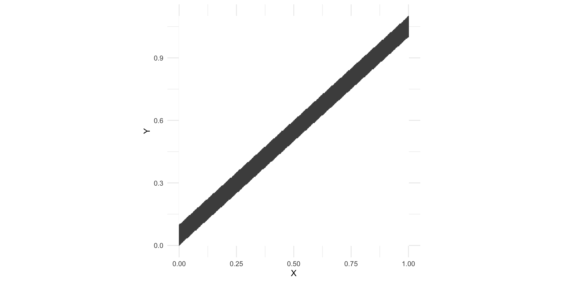
Example 1

In gray: the region where f_{X,Y}(x,y)>0

• When X increases, Y increases linearly (not surprising, since Y = X + Z)
• We expect the correlation \rho_{XY} to be close to 1

Example 1 – Computing \rho_{XY}

• For a random variable W \sim {\rm uniform} (a,b), we have {\rm I\kern-.3em E}[W] = \frac{a+b}{2} \,, \qquad {\rm Var}[W] = \frac{(b-a)^2}{12}

• Since X \sim {\rm uniform} (0,1) and Z \sim {\rm uniform} (0,1/10), we have {\rm I\kern-.3em E}[X] = \frac12 \,, \qquad {\rm Var}[X] = \frac{1}{12} \,, \qquad {\rm I\kern-.3em E}[Z] = \frac{1}{20} \,, \qquad {\rm Var}[Z] = \frac{1}{1200}

• Since X and Z are independent, we also have {\rm Var}[Y] = {\rm Var}[X + Z] = {\rm Var}[X] + {\rm Var}[Z] = \frac{1}{12} + \frac{1}{1200}

Example 1 – Computing \rho_{XY}

• Since X and Z are independent, we have {\rm I\kern-.3em E}[XZ] = {\rm I\kern-.3em E}[X]{\rm I\kern-.3em E}[Z]

• We conclude that \begin{align*} {\rm Cov}(X,Y) & = {\rm I\kern-.3em E}[XY] - {\rm I\kern-.3em E}[X] {\rm I\kern-.3em E}[Y] \\ & = {\rm I\kern-.3em E}[X(X + Z)] - {\rm I\kern-.3em E}[X] {\rm I\kern-.3em E}[X + Z] \\ & = {\rm I\kern-.3em E}[X^2] - {\rm I\kern-.3em E}[X]^2 + {\rm I\kern-.3em E}[XZ] - {\rm I\kern-.3em E}[X]{\rm I\kern-.3em E}[Z] \\ & = {\rm Var}[X] = \frac{1}{12} \end{align*}

Example 1 – Computing \rho_{XY}

• The correlation between X and Y is \begin{align*} \rho_{XY} & = \frac{{\rm Cov}(X,Y)}{\sqrt{{\rm Var}[X]}\sqrt{{\rm Var}[Y]}} \\ & = \frac{\frac{1}{12}}{\sqrt{\frac{1}{12}} \sqrt{ \frac{1}{12} + \frac{1}{1200}} } = \sqrt{\frac{100}{101}} \end{align*}

• As expected, we have very high correlation \rho_{XY} \approx 1

• This confirms a very strong linear relationship between X and Y

Example 2

• Assume X and Z are independent, and X \sim {\rm uniform} \left( -1,1 \right) \,, \qquad Z \sim {\rm uniform} \left( 0, \frac{1}{10} \right)

• Define the random variable Y = X^2 + Z

• Since X and Z are independent, and Z is uniform, we have that Y | X = x \, \sim \, {\rm uniform} \left( x^2, x^2 + \frac{1}{10} \right) (adding x^2 to Z simply shifts the uniform distribution of Z by x^2)

• Question: Is the correlation \rho_{XY} between X and Y high or low?

Example 2

• As Y | X \, \sim \, {\rm uniform} \left( X^2, X^2 + \frac{1}{10} \right), the conditional pdf of Y given X = x is f(y|x) = \begin{cases} 10 & \text{ if } \, y \in \left( x^2 , x^2 + \frac{1}{10} \right) \\ 0 & \text{ otherwise} \end{cases}

• As X \sim {\rm uniform} (-1,1), its pdf is f_X(x) = \begin{cases} \frac12 & \text{ if } \, x \in \left( -1 , 1 \right) \\ 0 & \text{ otherwise} \end{cases}

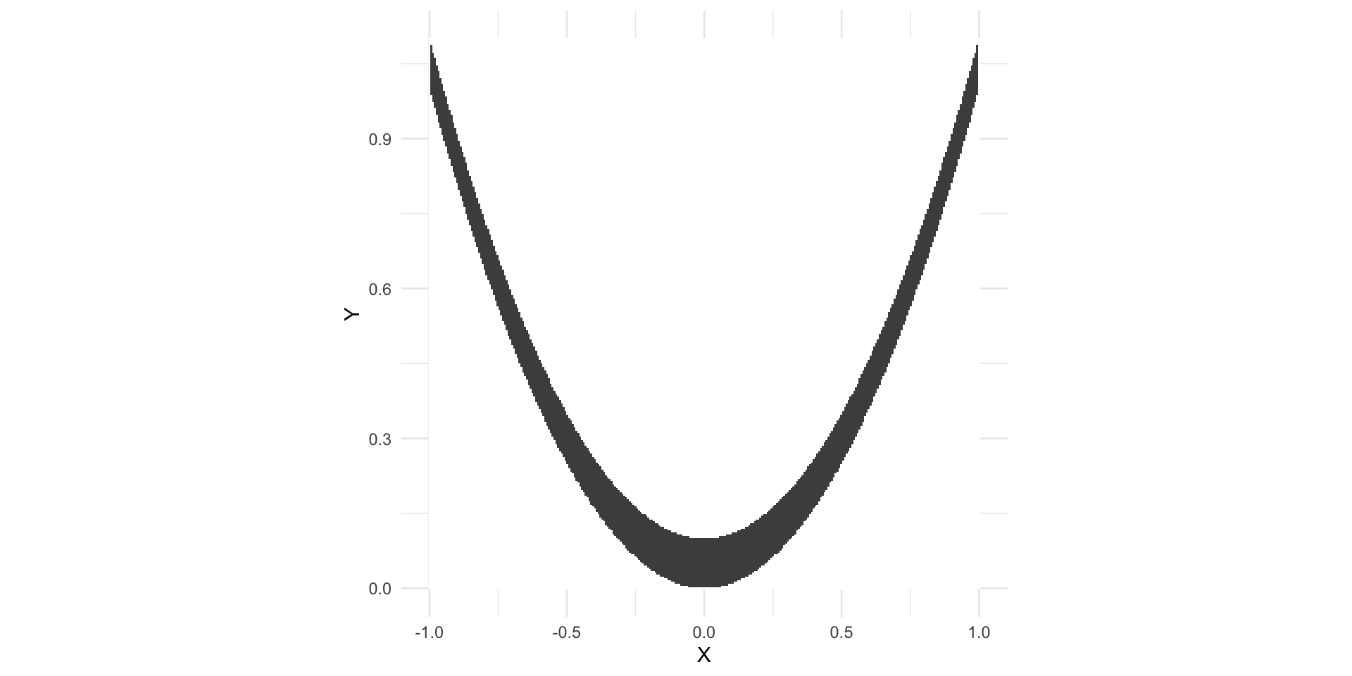
• Therefore, the joint distribution of (X,Y) is f_{X,Y}(x,y) = f(y|x)f_X(x) = \begin{cases} 10 & \text{ if } \, x \in (-1,1) \, \text{ and } \, y \in \left( x^2 , x^2 + \frac{1}{10} \right) \\ 0 & \text{ otherwise} \end{cases}

Example 2

In gray: the region where f_{X,Y}(x,y)>0

• When X increases, Y increases quadratically (not surprising, as Y = X^2 + Z)
• There is no linear relationship between X and Y \,\, \implies \,\, we expect \, \rho_{XY} \approx 0

Example 2 – Computing \rho_{XY}

• Since X \sim {\rm uniform} (-1,1), we can compute that {\rm I\kern-.3em E}[X] = {\rm I\kern-.3em E}[X^3] = 0

• Since X and Z are independent, we have {\rm I\kern-.3em E}[XZ] = {\rm I\kern-.3em E}[X]{\rm I\kern-.3em E}[Z] = 0

Example 2 – Computing \rho_{XY}

• Compute the covariance \begin{align*} {\rm Cov}(X,Y) & = {\rm I\kern-.3em E}[XY] - {\rm I\kern-.3em E}[X] {\rm I\kern-.3em E}[Y] \\ & = {\rm I\kern-.3em E}[XY] \\ & = {\rm I\kern-.3em E}[X(X^2 + Z)] \\ & = {\rm I\kern-.3em E}[X^3] + {\rm I\kern-.3em E}[XZ] = 0 \end{align*}

• The correlation between X and Y is \rho_{XY} = \frac{{\rm Cov}(X,Y)}{\sqrt{{\rm Var}[X]}\sqrt{{\rm Var}[Y]}} = 0

• This confirms there is no linear relationship between X and Y

References

[1]

Bingham, Nicholas H., Fry, John M., Regression, linear models in statistics, Springer, 2010.

[2]

Fry, John M., Burke, Matt, Quantitative methods in finance using R, Open University Press, 2022.

[3]

Casella, George, Berger, Roger L., Statistical inference, second edition, Brooks/Cole, 2002.

[4]

DeGroot, Morris H., Schervish, Mark J., Probability and statistics, Fourth Edition, Addison-Wesley, 2012.

[5]

Dalgaard, Peter, Introductory statistics with R, Second Edition, Springer, 2008.

[6]

Davies, Tilman M., The book of R, No Starch Press, 2016.