Statistical Models

Appendix C

Dr. Silvio Fanzon

S.Fanzon@hull.ac.uk

University of Hull

Appendix C:
Simulations & Bootstrap

Outline of Appendix C

1. Monte Carlo simulations
2. Simulating p-values
3. The Bootstrap

4. Bootstrap Confidence Intervals
5. Bootstrap t-test
6. Bootstrap F-test

Part 1:
Monte Carlo
simulations

For simple counts, we said that:

• The distribution of the \chi^2 statistic is approximately \chi^2 = \sum_{i=1}^n \frac{(O_i - E_i)^2 }{ E_i } \ \approx \ \chi_{n-1}^2

• The approximation is:

  Good	E_i \geq 5 \, \text{ for all } \, i = 1 , \ldots n
  Bad	E_i < 5 \, for some \, i = 1 , \ldots n

• How to compute the p-value: When approximation is

  • Good: Use \chi_{n-1}^2 approximation of \chi^2
  • Bad: Use Monte Carlo simulations

• Question: What is a Monte Carlo simulation?

Monte Carlo methods

• Monte Carlo methods:
  • Broad class of computational algorithms
  • They rely on repeated random sampling to obtain numerical results
  • Principle: use randomness to solve problems which are deterministic
• Why the name?
  • Method was developed by Stanislaw Ulam
  • His uncle liked to gamble in the Monte–Carlo Casino in Monaco
• Examples of applications:
  • First used to solve problem of neutron diffusion in Los Alamos 1946
  • Can be used to compute integrals
  • Can be used to compute p-values

Example: Approximation of \pi

• Throw random points inside square of side 2
• Count proportion of points falling inside unit circle
• Such proportion approximates \pi (area of the circle)
  • r = \, Red point
  • b = \, Blue point
  • n = r + b Total points

\frac{\pi}{4} \approx \frac{r}{n} \,\, \implies \,\, \pi \approx \frac{4r}{n}

Approximating \pi – Formal model

• Draw x_1, \ldots, x_N and y_1, \ldots, y_N from {\rm Uniform(-1,1)}

• Count the number of points (x_i,y_i) falling inside circle of radius 1

• These are points satisfying condition x_i^2 + y_i^2 \leq 1

• Area of circle estimated with proportion of points falling inside circle: \text{Area} \ = \ \pi \ \approx \ \frac{\text{Number of points } (x_i,y_i) \text{ inside circle}}{N} \ \times \ 4

• Note: 4 is the area of square of side 2

Plot: 1000 random points in square of side 2

Approximation of \pi in R

N <- 10000      # We do 100000 iterations and print every 10000
total <- 0      # Counts total number of points
in_circle <- 0  # Counts points falling in circle

for (j in 1:10) {   # This loop is for printing message every N iterations
  for (i in 1:N) {  # Loop in which points are counted
    x <- runif(1, -1, 1); y <- runif(1, -1, 1);  # sample point (x,y)
    if (x^2 + y^2 <= 1) {    
      in_circle <- in_circle + 1  # If (x,y) in circle increase counter
    }
    total <- total + 1  # Increase total counter (in any case)
  }
  
  pi_approx <- ( in_circle / total ) * 4  # Compute approximate area

  cat(sprintf("After %8d iterations pi is %.08f, error is %.08f\n",
     (j * N), pi_approx, abs(pi_approx - pi)))
}

• The R code can be downloaded here monte_carlo_pi.R

Approximation of \pi in R: Output

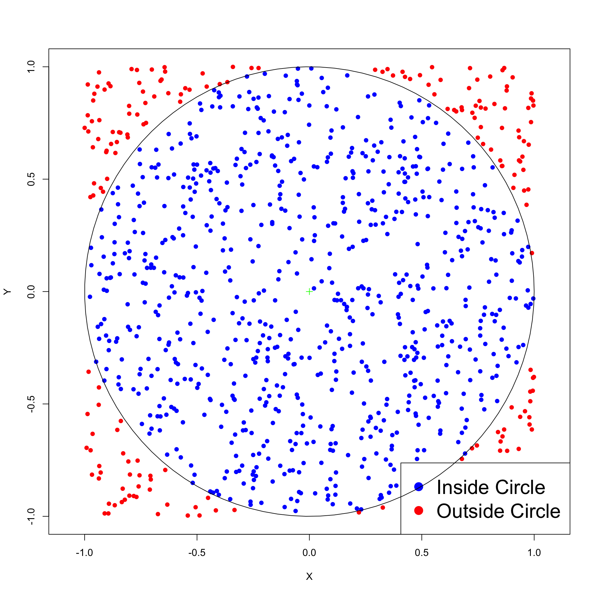
After    10000 iterations pi is 3.14560000, error is 0.00400735
After    20000 iterations pi is 3.13260000, error is 0.00899265
After    30000 iterations pi is 3.13253333, error is 0.00905932
After    40000 iterations pi is 3.14170000, error is 0.00010735
After    50000 iterations pi is 3.14248000, error is 0.00088735
After    60000 iterations pi is 3.14186667, error is 0.00027401
After    70000 iterations pi is 3.14200000, error is 0.00040735
After    80000 iterations pi is 3.14155000, error is 0.00004265
After    90000 iterations pi is 3.14177778, error is 0.00018512
After   100000 iterations pi is 3.14084000, error is 0.00075265

Note:

• The error decreases overall, but there are random fluctuations

• This is because we are trying to approximate \pi by a random quantity

A word on error estimates

• Deriving error estimates for numerical methods is not easy (Numerical Analysis)

• Going back to our example:

  • Let n denote the total number of points drawn
  • Let X_n denote the proportion of points falling inside the unit circle

• For every \varepsilon> 0 fixed, it can be shown that P( | X_n - \pi/4 | \geq \varepsilon) \leq {\rm Error} = \frac{1}{20 n \varepsilon^2}

• To get small Error: \,\, \varepsilon has to be small, n has to be large

  • Fixing a small error threshold \varepsilon implies doing more iterations (larger n)
  • Error estimate is probabilistic: Error fluctuates, but decreases with more iterations

• Estimate can be derived by interpreting the problem as the Monte Carlo integration of \int_0^1 \sqrt{1-x^2} \, dx = \pi /4, see stackexchange post

Simulation: The main point (for us)

Simulation can be used to gain insight into the shape of a distribution:

• Mean and variance

• Related probabilities (p-values)

How to simulate in R:

• Use loops
  • Example: We used a for loop to simulate \pi
• Use ad hoc R commands
  • replicate(n, expr) repeats expression n times and outputs results
  • apply(x, expr) applies expression to the object x

Example: Estimating mean / variance of \overline{X}

Consider sample X_1, \ldots, X_n from N(\mu,\sigma^2)

• Recall that the sample mean satisfies {\rm I\kern-.3em E}[\overline{X}] = \mu \,, \qquad {\rm Var}[\overline{X}] = \frac{\sigma^2}{n} (As n gets larger, {\rm Var}[\overline{X}] will be closer to 0 \implies \overline{X} \approx \mu when n is large)

• For example, if the sample size is n = 10, mean \mu = 0 and sd \sigma = 1, then {\rm I\kern-.3em E}[\overline{X}] = 0 \,, \qquad {\rm Var}[\overline{X}] = \frac{1}{10} = 0.1

• We can obtain the above quantitites through simulation
  (In fancy terms: Estimating mean and variance of \overline{X})

• One simulation of \overline{X} can be done as follows:
  1. Generate sample x_1, \ldots, x_n from N(0,1)
  2. Compute sample mean of x_1, \ldots, x_n

# Simulate the sample mean xbar

n <- 10
sim.xbar <- mean(rnorm(n)) 

• To simulate M = 1000 values from \overline{X}, replicate the above command M times

# Simulate M = 1000 times the sample mean xbar
n <- 10; M <- 1000

sim.xbar <- replicate(M, mean(rnorm(n)))

• The vector sim.xbar contains M=1000 simulations from \overline{X}

• Reasonable to suppose that sim.xbar approximates the random variable \overline{X}
  (This can be made rigorous with Central Limit Thm)

• Therefore, we can make the following estimation

Quantity	Estimation
{\rm I\kern-.3em E}[\overline{X}]	Sample mean of sim.xbar
{\rm Var}[\overline{X}]	Sample variance of sim.xbar

# Print mean and variance of sample mean
cat("Expected value:", mean(sim.xbar), "Variance:", var(sim.xbar))

Expected value: 0.005180686   Variance: 0.1058328

These are very close to the theoretical values: \quad {\rm I\kern-.3em E}[\overline{X}] = 0 \,, \quad {\rm Var}[\overline{X}] = \frac{1}{10} = 0.1

Example: Sample mean VS sample median

• Both sample mean and median can be used to estimate the center of a distribution

• But which one is better?

• Suppose the population is N(\mu,\sigma^2)

• We know that the sample mean \overline{X} satisfies {\rm I\kern-.3em E}[\overline{X}] = \mu \,, \qquad {\rm Var}[\overline{X}] = \frac{\sigma^2}{n}

• However, no such formulas are available for the sample meadian

Question: How can we compare them? Use simulation

To simulate sample mean and median from N(0,1), we do:

• Generate sample x_1, \ldots, x_{10} from N(0,1), and compute sample mean and median

• Repeat M = 1000 times

M <- 1000; n <- 10  
sim.mean <- replicate(M, mean(rnorm(n)))
sim.median <- replicate(M, median(rnorm(n)))

• To compare simulated sample mean and median, we can produce a boxplot

• The one with smallest variance, will be the better estimator for the true population mean \mu = 0

boxplot(list("sample mean" = sim.mean, 
             "sample median" = sim.median),
        main = "Normal population N(0,1)")

• The sample mean has less variability
• It is the preferred estimator for the true population mean
  (when the population is normal)

Example: Computing probabilities

Question: What is the probability of rolling 7 with two dice?

• Of course this problem has combinatorial answer: p = \frac16

• But we can also answer using simulation

• To simulate the roll of a dice, we use the function sample

  • sample(x, n, replace = T)
  • samples n times from vector x with replacement

• To roll 2 dice, we input:

# Roll two dice

sample(1:6, 2, replace = T)

[1] 3 1

To compute the probability of rolling 7 with two dice we do:

• Simulate one roll of the two dice, and sum the outcome
• Repeat M = 1000 times
• Estimate the probability of rolling a 7 with P(\text{Rolling } 7) \approx \frac{\# \text{ of times the simulated roll is } 7 }{1000}

M <- 1000

sim.rolls <- replicate(M, sum( sample(1:6, 2, replace = T) ))

number.of.7s <- sum( sim.rolls == 7 )
p <- number.of.7s / M

cat("The estimated probability of rolling 7 is", p)

The estimated probability of rolling 7 is 0.166

• This is very close to the theoretical probability p = 1/6

Example: Interpretation of Confidence Intervals

• Suppose given a normal population N(\mu,\sigma^2)

• A 95 \% confidence interval for the true mean \mu is a (random) interval [a,b] s.t. P(\mu \in [a,b]) = 0.95

• Confidence interval is not probability statement about \mu – note \mu is a constant!

• It is probability statement about [a,b]

Interpretation: The random interval [a,b] contains the mean \mu with probability 0.95

Constructing the confidence interval with t-statistic:

• Suppose given a sample x_1, \ldots, x_n from N(\mu,\sigma^2)

• Recall: the t-statistic has t-distribution t = \frac{\overline{x}-\mu}{\mathop{\mathrm{e.s.e.}}} \, \sim \, t_{n-1} \,, \qquad \mathop{\mathrm{e.s.e.}}= \frac{s}{\sqrt{n}}

• We impose that t is observed with probability 0.95 P(- t^* \leq t \leq t^*) = 0.95 \,, \qquad t^* = t_{n-1}(0.025)

• The 95\% confidence interval is obtained by solving above equation for \mu P(\mu \in [a,b] ) = 0.95 \,, \qquad a = \overline{x} - t^* \times \mathop{\mathrm{e.s.e.}}, \qquad b = \overline{x} + t^* \times \mathop{\mathrm{e.s.e.}}

• Interpretation: If you sample over and over again, the interval [a,b] will contain \mu about 95\% of the times

• Each row of points is a sample from the same normal distribution \qquad (Image from Wikipedia)

• The colored lines are confidence intervals for the mean \mu

• At the center of each interval is the sample mean (diamond)

• The blue intervals contain the population mean, and the red ones do not

Simulating one confidence interval in R:

• Sample n = 100 times from N(0,1)
  • Running a t-test on the sample gives a confidence interval for the unknown mean \mu
  • The confidence interval can be retrieved with $conf.int

# Sample 100 times from N(0,1)
x <- rnorm(100)

# Compute confidence interval using t.test
interval <- t.test(x)$conf.int

• interval is a vector containing the simulated confidence interval
  • Left extreme in interval[1] \qquad Right extreme in interval[2]

a <- interval[1];   b <- interval[2]

cat("Simulated confidence interval: a =", a, "  b = ", b)

Simulated confidence interval: a = -0.2262375   b =  0.1689576

• In this case the interval contains the true mean \mu = 0

Testing the claim: \quad P (\mu \in [a,b]) = 0.95

• If you sample over and over, the interval [a,b] will contain \mu about 95\% of the times

We test with the following method:

• Sample n = 100 times from N(0,1) and compute confidence interval

• Repeat M = 1000 times

• Check how many times \mu = 0 belongs to simulated confidence intervals

• Estimate the probability of the CI containing \mu as P(\mu \in [a,b]) \approx \frac{\# \text{ of times } \mu = 0 \text{ belongs to simulated } [a,b]}{M}

• The estimate should approach 0.95

• First, we simulate the M = 1000 confidence intervals

# Simulate M confidence intervals for the mean
n <- 100; M <- 10000

intervals <- replicate(M, t.test(rnorm(n)) $ conf.int)

• intervals is a matrix containing the M = 1000 simulated intervals (as columns)
  • Left extremes are in intervals[1, ]
  • Right extremes are in intervals[2, ]
• For visualization, we print the first 5 confidence intervals

# Print the first 5 columns of intervals
intervals[ ,1:5]

           [,1]        [,2]       [,3]       [,4]        [,5]
[1,] -0.2262375 -0.07222545 -0.2428610 -0.1788659 -0.07420973
[2,]  0.1689576  0.35116698  0.1201007  0.2189942  0.30661995

• Now, we have our M = 1000 confidence intervals for \mu = 0

• Check how many times \mu = 0 belongs to simulated confidence intervals

# Save left and right extremes in vectors
a <- intervals[1, ];   b <- intervals[2, ]

# Check how many times mu = 0 belongs to (a,b)
mu.belongs <- sum( (a < 0) & (0 < b) )

# Estimate the probability that mu = 0 belongs to (a,b)
p <- mu.belongs / M

cat("mu = 0 belongs to the confidence interval with probability", p)

mu = 0 belongs to the confidence interval with probability 0.9494

• This approximates the theoretical probability P(\mu \in [a,b]) = 0.95 (we would need more confidence intervals for a better estimate)

Part 2:
Simulating p-values

The problem of simulating p-values

Suppose given a random variable X such that

• The distribution of X is (possibly) unknown

• A method for simulating X is available

  • This means we can (somehow) sample values from X

Goal: For a given x^*, we want to estimate the p-value

p = P(X > x^*)

General recipe to simulate p-values

Goal: Estimate the p-value p = P(X>x^*)

1. Simuate the random varible X. You obtain a numerical value X_{\rm sim}

2. The simulated value is extreme if X_{\rm sim} > x^*

3. There are two possibilities:

   • X_{\rm sim} is extreme \quad \,\,\, \quad \implies \quad simulation goes in favor of \, p
   • X_{\rm sim} is not extreme \quad \implies \quad simulation goes in favor of \, 1-p

4. We estimate the p-value as p = P( X > x^* ) \ \approx \ \frac{ \# \text{ of extreme simulated values} }{ \text{Total number of simulations} }

Example: Monte Carlo p-value for goodness-of-fit test

Goal: use Monte Carlo simulations to compute p-value for goodness-of-fit test

• Consider data counts

Type	1	\ldots	n	Total
Observed counts	o_1	\ldots	o_n	m
Null Probabilities	p_1^0	\ldots	p_n^0	1

• The expected counts are E_i = m p_i^0

• Under the null hypothesis, the observed counts (o_1, \ldots, o_n) come from (O_1 , \ldots, O_n) \sim \mathop{\mathrm{Mult}}(m, p_1^0, \ldots, p_n^0)

p-value for goodness-of-fit test

• The chi-squared statistic random variable is \chi^2 = \sum_{i=1}^n \frac{(O_i - E_i)^2 }{ E_i }

• The observed chi-squared statistics is \chi^2_{\rm obs} = \sum_{i=1}^n \frac{(o_i - E_i)^2 }{ E_i }

• The p-value is defined as p = P( \chi^2 > \chi^2_{\rm obs} )

Problem: Computing p-value for low counts

• Suppose E_i < 5 for some i

• In this case, \chi^2 is not \chi^2_{n-1} distributed

• In fact, the distribution is unknown \chi^2 = \sum_{i=1}^n \frac{(O_i - E_i)^2 }{ E_i } \ \, \sim \ \, ???

• If the distribution is unknown, how do we compute the p-value p = P( \chi^2 > \chi^2_{\rm obs} ) \ \ ???

Exercise: Come up with a simulation to approximate p

Method: Simulating p-value for \chi^2 statistic

1. Simulate counts (o_1^{\rm sim},\ldots,o_n^{\rm sim}) from \mathop{\mathrm{Mult}}(m, p_1^0, \ldots, p_n^0)

2. Compute the corresponding simulated chi-squared statistic \chi^2_{\rm sim} = \sum_{i=1}^n \frac{ (o_i^{\rm sim} - E_i)^2 }{E_i} \,, \qquad E_i := m p_i^0

3. The simulated chi-squared statistic is extreme if \chi^2_{\rm sim} > \chi^2_{\rm obs} \,, \quad \text{ where \, } \chi^2_{\rm obs} = \sum_{i=1}^n \frac{(o_i - E_i)^2 }{ E_i } \,, \,\, o_i \, \text{ the observed counts}

4. We estimate the theoretical p-value by p = P( \chi^2 > \chi^2_{\rm obs} ) \ \approx \ \frac{ \# \text{ of extreme simulated statistics} }{ \text{Total number of simulations} }

Exercise

Data: Number of defects in printed circuit boards, along with null probabilities

# Defects	0	1	2	3
Counts	32	15	9	4
Null Probabilities	0.5	0.3	0.15	0.05

• Total number of counts is m = 60. Expected counts are E_i = m p_i^0

E_1	E_2	E_3	E_4
30	18	9	3

• Note: E_4 = 3 < 5 \quad \implies \quad the distribution of \chi^2 is unknown

• Exercise: Write R code to perform a goodness-of-fit test on above data

  • You may not use the function chisq.test
  • p-value should be simulated (see previous slide)

Solution

• First, compute the observed chi-squared statistic:
  • Enter observed counts and null probabilities
  • Compute total counts, expected counts and \chi^2_{\rm obs}

# Enter counts and null hypothesis probabilities
counts <- c(32, 15, 9, 4)
null.p <- c(0.5, 0.3, 0.15, 0.05)

# Compute total counts
m <- sum(counts)

# Compute expected counts
exp.counts <- m * null.p

# Compute the observed chi-squared statistic
obs.chi <- sum( (counts - exp.counts)^2 / exp.counts )

We now generate M = 10000 simulated chi-squared statistics:

1. Simulate counts (o_1^{\rm sim},\ldots,o_n^{\rm sim}) from \mathop{\mathrm{Mult}}(m, p_1^0, \ldots, p_n^0)

2. Compute the corresponding simulated chi-squared statistic \chi^2_{\rm sim} = \sum_{i=1}^n \frac{ (o_i^{\rm sim} - E_i)^2 }{E_i}

# Simulate M chi-squared statistics
M <- 10000

sim.chi <- replicate(M, {
                # Simulate multinomial counts under null hypothesis
                sim.counts <- rmultinom(1, m, null.p)
                            
                # Return chi-squared statistic from the simulated counts
                sum( (sim.counts - exp.counts )^2 / exp.counts)
                })

• The vector sim.chi contains M = 10000 simulated chi-squared statistics

• We approximate the p-value by p = P(\chi^2 > \chi_{\rm obs}^2) \approx \ \frac{ \# \text{ of extreme simulated statistics} }{ M }

# Check how many simulated statistics are extreme
num.extreme <- sum( sim.chi > obs.chi )

# Estimate the p-value
sim.p.value <- num.extreme / M

• As cross check, we also simulate the p-value with chisq.test

# Perform chi-squared test using built-in R function
ans <- chisq.test(counts, p = null.p, simulate.p.value = T)

# Extract p-value from chi-squared test result
R.p.value <- ans$p.value

# Print p-values for comparison
cat("\nOur simulated p-value is:", sim.p.value)
cat("\nR simulated p-value is:", R.p.value)

Our simulated p-value is: 0.8169

R simulated p-value is: 0.8195902

• Note: The simulated p-values are the same! (up to random fluctuations)

• Conclusion: We see that p > 0.05. There is not enough evidence to reject H_0

Part 3:
The Bootstrap

Motivation

• So far, our simulations used knowledge of the population distribution, e.g.

  • To simulate \pi, we sampled points from {\rm Uniform}([-1,1] \times [-1,1])
  • To simulate the \chi^2 statistic, we sampled Multinomial counts
  • To simulate confidence intervals, we sampled from a normal population

• Problem: Sometimes the population distribution f is unknown

• Bootstrap: Replace the unknown distribution f with a known distribution \hat{f}

The Sample Distribution

• Assume given a sample x_1,\ldots,x_n from a population f

• The Sample Distribution is the discrete distribution which puts mass \frac1n at each sample point \hat{f}(x) = \begin{cases} \frac1n & \quad \text{ if } \, x \in \{x_1, \ldots, x_n\} \\ 0 & \quad \text{ otherwise } \end{cases}

Theorem: Glivenko-Cantelli

As the sample size increases \lim_{n \to \infty} \hat{f} = f

(more precisely, the convergence is uniform almost everywhere wrt the cdfs: \hat{F} \to F)

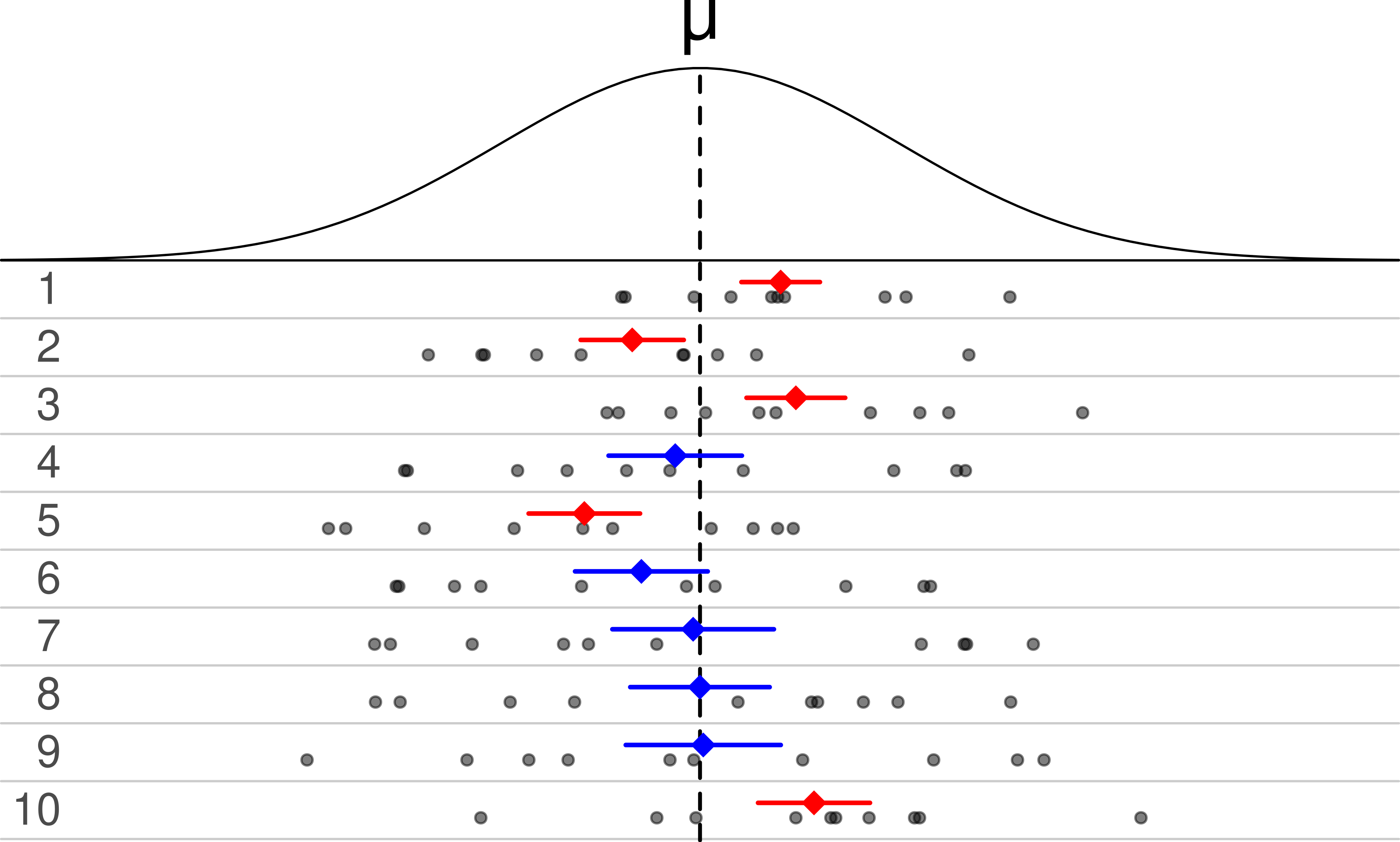
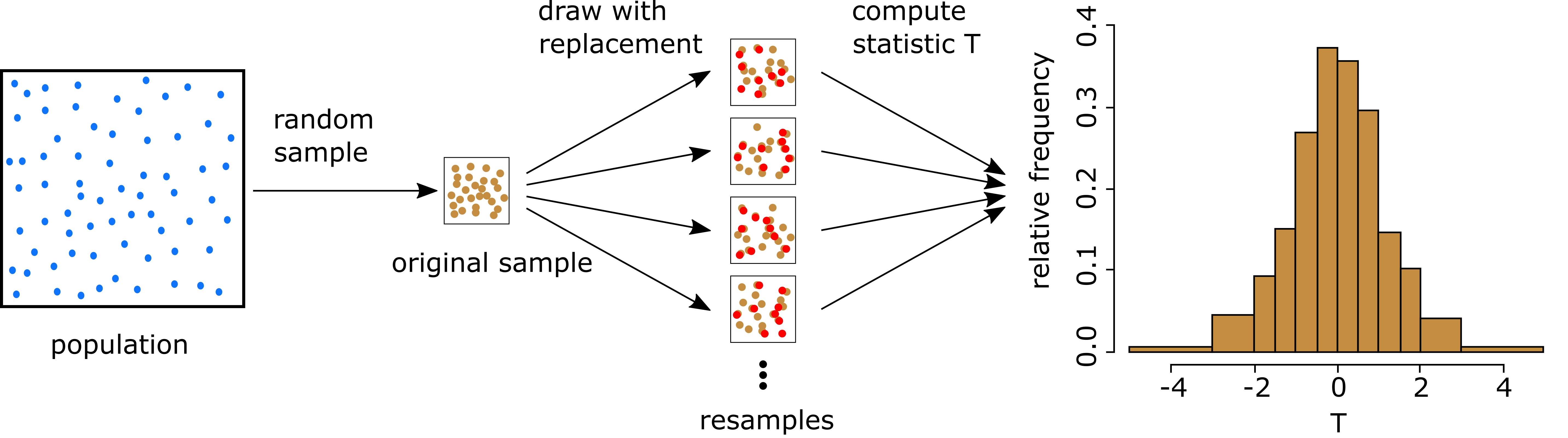
Main Bootstrap idea

Setting: Assume given the original sample x_1,\ldots,x_n from unknown population f

Bootstrap: Regard the sample as the whole population

• Replace the unknown distribution f with the sample distribution \hat{f}(x) = \begin{cases} \frac1n & \quad \text{ if } \, x \in \{x_1, \ldots, x_n\} \\ 0 & \quad \text{ otherwise } \end{cases}

• Any sampling will be done from \hat{f} \qquad \quad (motivated by Glivenko-Cantelli Thm)

Note: \hat{f} puts mass \frac1n at each sample point

Drawing an observation from \hat f is equivalent to drawing one point at random from the original sample \{x_1,\ldots,x_n\}

The Bootstrap Algorithm

Setting: Given the original sample x_1,\ldots,x_n from unknown population f

Bootstrap Algorithm: to estimate the distribution of a statistic of interest T

1. Draw sample x_1^*,\ldots,x_n^* from \{x_1, \ldots, x_n\} with replacement

2. Compute the statistic T on the bootstrap sample T^* = T(x_1^*,\ldots,x_n^*)

3. Repeat Steps 1 and 2, B times, to get B bootstrap simulations of T T^*_1, \ldots , T^*_B These values represent the bootstrap distribution of T

Note: If population distribution f is known, we would just sample from f

• Original sample \{x_1,\ldots,x_n\} is drawn from the population \qquad (Image from Wikipedia)

• Resamples \{x_1^*,\ldots,x_n^*\} are generated by drawing from \{x_1,\ldots,x_n\} with replacement

• Note: Data points x_i can be drawn more than once (in red and sligthly offsetted)

• For each resample, the statistic T^* is calculated

• Therefore, a histogram can be calculated to estimate the bootstrap distribution of T

Q & A

References?

• Simulation and bootstrap are huge topics

• Good introduction: the book by Efron (inventor of bootstrap) and Tibshirani [1]

Why is the Bootstrap useful?

• Because a lot of the times population distribution is unknown

• Despite this, bootstrap allows to do inference on statistic T

Why does the Bootstrap work? We are just resampling from the original sample!

• It (often) works because the original sample encodes population variability

• By resampling the original sample, we are simulating this variability

Q & A

How good is the bootstrap distribution of T?

• It can be a good approximation of the true distribution of T when the
  original sample is sufficiently variable
  • Things tend to go well for large samples (n \geq 50)
• Bootstrap works well when the statistic T is a mean (or something like a mean)
  • for example median, regression coefficient, or standard deviation.
• The bootstrap has difficulties when the statistic T is influenced by outliers
  • for example if T is the range, that is, T = max value - min value

Q & A

What are the limitations of bootstrap?

• Computationally expensive
  • For decent simulation of bootstrap distribution of T, need at least
    B = 10,000 resamples (100,000 would be better!)
• Relies on a sufficiently variable original sample
  • If the original sample is not good, the bootstrap cannot recover from this problem
  • In this case the bootstrap population will not look like the true population
  • The bootstrap resampling will not be useful
• No way to determine if the original sample is good enough

However, problems are usually mitigated by large enough original sample (n \geq 50)

Example: Bootstrapping the mean

Setting: Given the original sample x_1,\ldots,x_n from unknown population f

Bootstrap Algorithm: to estimate the distribution of the sample mean \overline{X}

1. Draw sample x_1^*,\ldots,x_n^* from \{x_1, \ldots, x_n\} with replacement

2. Compute the sample mean \overline{X} on the bootstrap sample \overline{X}^* = \frac{1}{n} \sum_{i=1}^n x_i^*

3. Repeat Steps 1 and 2, B times, to get B bootstrap simulations of \overline{X}^* \overline{X}^*_1, \ldots , \overline{X}^*_B These values represent the bootstrap distribution of \overline{X}

Implementation in R

• Store the original sample into a vector and compute length

# Store original sample and compute length

x <- c(x_1, ..., x_n)
n <- length(x)

• To generate one bootstrap simulation of \overline{X}:
  1. Sample n times from \{x_1,\ldots,x_n\} with replacement
  2. This gives the bootstrap sample \{x_1^*,\ldots,x_n^*\}
  3. Compute sample mean of the bootstrap sample

# Bootstrap sample mean one time
x.star <- sample(x, n, replace = TRUE)     # Sample n times with replacement
xbar.star <- mean(x.star)

• To generate B = 10,000 bootstrap simulations of \overline{X}, use replicate

# Bootstrap sample mean B = 10,000 times
B <- 10000

xbar.star <- replicate(B, {
                       # Generate bootstrap sample
                       x.star <- sample(x, n, replace = TRUE)
                       # Return mean of bootstrap sample
                       mean(x.star)
                      })

• The vector xbar.star contains B = 10,000 bootstrap samples of \overline{X}

Why is this useful?: When the population is normal N(\mu,\sigma^2), we know that \overline{X} \sim N(\mu, \sigma^2/n) However: population distribution unknown \implies distribution of \overline{X} unknown

Bootstrap gives a way to estimate distribution of \overline{X}

Worked Example

Original sample: CEOs compensation in 2012 (USA data - in million dollars)

CEO Pay 2012

23.5

6.4

11.1

3.8

8.9

4.8

23.8

3.0

2.9

3.2

We want to simulate the bootstrap distribution of the sample mean \overline{X}

• To do so, we generate B = 10,000 bootstrap simulations of sample mean \overline{X}

# Enter original sample and compute size
x <- c(23.5, 6.4, 11.1, 3.8, 8.9, 4.8, 23.8, 3, 2.9, 3.2)
n <- length(x)

# Bootstrap sample mean B = 10,000 times
B <- 10000

xbar.star <- replicate(B, {
                       # Generate bootstrap sample
                       x.star <- sample(x, n, replace = TRUE)
                       # Return mean of bootstrap sample
                       mean(x.star)
                      })

• The vector xbar.star contains B = 10000 bootstrap samples from \overline{X}

• We can examine the bootstrap distribution of \overline{X} with a histogram

  • If population was normal, we would expect \overline{X} to be normal
  • However \overline{X} is skewed to the right \implies population might not be normal

hist(xbar.star)

• Plotting the density of x shows that the data is heavily skewed (not normal)

plot(density(x))

Part 4:
Bootstrap CI

Bootstrap Confidence Intervals

• When the population is normally distributed N(\mu,\sigma^2), we used the t-statistic t = \frac{\overline{x} - \mu}{\mathop{\mathrm{e.s.e.}}} to form a (1-\alpha)100\% confidence interval [a,b] for the population mean \mu P(\mu \in [a,b]) = 1-\alpha \,, \quad a, b = \overline{x} \mp t^* \times \mathop{\mathrm{e.s.e.}}, \quad t^* = t_{n-1}\left(\frac{\alpha}{2}\right)

• If the population is not normal, the interval [a,b] might not be accurate, meaning that P(\mu \in [a,b]) \neq 1 - \alpha

• In this case, the bootstrap sample mean can be used to form a CI

• Moreover, bootstrap CI easily generalize to any estimator T

Algorithm: Bootstrap Confidence Intervals

Setting: Given the original sample x_1,\ldots,x_n from unknown population f, and

• \theta population parameter \,\, (e.g. \, \theta = mean), \,\, T estimator for \theta \,\, (e.g. \, T = sample mean)

Bootstrap CI Algorithm: to simulate (1-\alpha)100\% CI for parameter \theta

1. Bootstrap B times the statistic T, obtaining the bootstrap simulations T^*_1, \ldots , T^*_B

2. Order the values T^*_1, \ldots , T^*_B to obtain T^*_{(1)} \leq \ldots \leq T^*_{(B)}

3. Let \, m = [(\alpha/2)B], where [\cdot] is the ceiling function. The percentile bootstrap CI for \theta is \left[ T^*_{(m)} , T^*_{(B + 1- m)} \right] Endpoints are \frac{\alpha}{2}100\% and (1 − \frac{\alpha}{2})100\% percentiles of sample distribution of T^*_1, \ldots , T^*_B

Worked Example 1

Original sample:

• A consumer group wishes to see whether the actual mileage of a new SUV matches the advertised 17 miles per gallon

• To test the claim, the group fills the SUV’s tank and records the mileage

• This is repeated 10 times. The results are below

mpg

11.4

13.1

14.7

14.7

15.0

15.5

15.6

15.9

16.0

16.8

We want to simulate 95\% bootstrap CI for the population mean \mu

• First, we generate B = 10,000 bootstrap simulations of sample mean \overline{X}

# Enter original sample and compute size
x <- c(11.4, 13.1, 14.7, 14.7, 15.0, 15.5, 15.6, 15.9, 16.0, 16.8)
n <- length(x)

# Bootstrap sample mean B = 10,000 times
B <- 10000

xbar.star <- replicate(B, mean( sample(x, n, replace = TRUE) ))

• The vector xbar.star contains B = 10000 bootstrap samples from \overline{X}

• The (1-\alpha)\% bootstrap CI for the population mean \mu is \left[ \overline{X}^*_{(m)} , \overline{X}^*_{(B + 1- m)} \right]\,, \qquad m = [(\alpha/2)B]

• We have B = 10,000 and \alpha = 0.05 \quad \implies \quad m = 250

• Therefore, the 95\% bootstrap CI for the population mean \mu is \left[ \overline{X}^*_{(250)} , \overline{X}^*_{(9751)} \right]

• These percentiles can be automatically computed using the quantile function

# Compute 95% CI from bootstrap samples
alpha <- 0.05
boot.CI <- quantile(xbar.star, probs = c(alpha/2, 1-alpha/2))

• We compare the bootstrap CI to the usual t-statistic CI

# Compute 95% t-statistic CI
t.stat.CI <- t.test(x)$conf.int

# Print results
cat("Bootstrap Confidence Interval (95%):", boot.CI)
cat("\nt-statistic Confidence Interval (95%):", t.stat.CI)

Bootstrap Confidence Interval (95%): 13.86 15.71

t-statistic Confidence Interval (95%): 13.74545 15.99455

• The CI are almost overlapping

• This is a very strong indication that the original population is normal

  • Indeed, this is the case: You can verify it by plotting the density of mpg

• The advertised 17 mpg do not fall in either CI. We have reason to doubt the claim

• The code can be downloaded here bootstrap_CI.R

Worked Example 2

Original sample: Compensation data for a sample of CEOs in 2012
(USA data, in million dollars)

CEO Pay 2012

23.5

6.4

11.1

3.8

8.9

4.8

23.8

3.0

2.9

3.2

We want to simulate 95\% bootstrap CI for the mean compensation \mu

ceo12 <- c(23.5, 6.4, 11.1, 3.8, 8.9, 4.8, 23.8, 3, 2.9, 3.2)
plot(density(ceo12))

• Plotting the density of ceo12, we see that the data is not normal
  • Therefore, CI based on t-statistic would not be appropriate
  • Need to compute a Bootstrap CI for \mu

• Running the code bootstrap_CI.R on the new data, we get

# Enter original sample and compute size
x <- c(23.5, 6.4, 11.1, 3.8, 8.9, 4.8, 23.8, 3, 2.9, 3.2)
n <- length(x)

# Bootstrap sample mean B = 10,000 times
B <- 10000

xbar.star <- replicate(B, mean( sample(x, n, replace = TRUE) ))

# Compute 95% CI from bootstrap samples
alpha <- 0.05
boot.CI <- quantile(xbar.star, probs = c(alpha/2, 1-alpha/2))

# Compute 95% t-statistic CI
t.stat.CI <- t.test(x)$conf.int

# Print results
cat("Bootstrap Confidence Interval (95%):", boot.CI, 
"\nt-statistic Confidence Interval (95%):", t.stat.CI)

Bootstrap Confidence Interval (95%): 4.84 14.4005 
t-statistic Confidence Interval (95%): 3.339166 14.94083

• The bootstrap and t-statistic CI differ considerably, especially at low end

• Bootstrap CI has to be preferred, due to non-normality of data

Part 5:
Bootstrap t-test

Motivation

• Compensation data for a sample of CEOs in 2012 and 2013
  (USA data, in million dollars)

CEO Pay 2013	3.2	3.8	2.6	3.5	7.0	20.4	7.5	3.4	5.0	6.0
CEO Pay 2012	23.5	6.4	11.1	3.8	8.9	4.8	23.8	3.0	2.9	3.2

• Want to test for a difference in means via the t-statistic t = \frac{\bar{x} -\bar{y}}{s_p\sqrt{\frac{1}{n}+\frac{1}{m}}} \,, \qquad s_p = \sqrt{\frac{s^2_X(n-1)+s^2_Y(m-1)}{n+m-2}}

• Want to test for a difference in variance via the F-statistic F=\frac{s_X^2}{s_Y^2}

Motivation

• Compensation data for a sample of CEOs in 2012 and 2013
  (USA data, in million dollars)

CEO Pay 2013	3.2	3.8	2.6	3.5	7.0	20.4	7.5	3.4	5.0	6.0
CEO Pay 2012	23.5	6.4	11.1	3.8	8.9	4.8	23.8	3.0	2.9	3.2

• Under assumptions of normality and independence of the populations, we have t \sim t_{n+m-2} \,, \qquad F \sim F_{n-1,m-1}

• This information allows to compute the exact p-values for the t and F tests p_t = 2 P( t_{n+m-2} > |t| ) \,, \qquad p_F = 2P(F_{n-1,m-1} > F )

• Question: What if we cannot assume normality? How do we compute p-values?

• Answer: Bootstrap p-values

  • like simulated p-values, but sampling from the sample, instead of the population

Bootstrap t-test procedure

• Suppose given two samples:

  • x_1, \ldots, x_n from a population with cdf F(x)
  • y_1, \ldots, y_m from a population with cdf F(x - \Delta)

• Note: Population distributions have the same shape

  • Same spread, but they are shifted by \Delta \in \mathbb{R}

• Denoting by \mu_X and \mu_Y the means of F(x) and F(x - \Delta), we have \Delta = \mu_X - \mu_Y

• We want to test for difference in means H_0 \colon \mu_X = \mu_Y \,, \quad \qquad H_1 \colon \mu_X \neq \mu_Y , \quad \mu_X < \mu_Y \,, \quad \text{ or } \quad \mu_X > \mu_Y

• We are not making assumptions on F \implies distribution of t-statistic is unknown

  • Need to bootstrap the t-statistic

• Assume the null hypothesis is true: \mu_X = \mu_Y \quad \implies \quad \Delta = \mu_X - \mu_Y = 0

• Hence, under H_0, the two samples come from the same population F

• This means the two samples are actually part of a single sample of size n+m \mathcal{S} = \{x_1, \ldots, x_n , y_1, \ldots, y_m \}

• The sample distribution \hat{F} of \mathcal{S} is an approximation of F
  (Glivenko-Cantelli Theorem)

• We can therefore bootstrap the t-statistic from the combined sample \mathcal{S}

• The bootstrap samples are generated as follows:

  • Sample \{x_1^*, \ldots, x_n^*\} from \mathcal{S} with replacement
  • Sample \{y_1^*, \ldots, y_m^*\} from \mathcal{S} with replacement

• Compute a bootstrap simulation of the t-statistic t^* = \frac{\bar{x}^* -\bar{y}^*}{s_p\sqrt{\frac{1}{n}+\frac{1}{m}}} \,, \qquad s_p = \sqrt{\frac{(s^2_X)^*(n-1)+(s^2_Y)^*(m-1)}{n+m-2}}

• Repeat B times to obtain t^*_1, \ldots , t^*_B

• These values represent the bootstrap distribution of the t-statistic

• We now compare the bootstrap t-statistic to the observed statistic t_{\rm obs} = \frac{\bar{x} -\bar{y}}{s_p\sqrt{\frac{1}{n}+\frac{1}{m}}} \,, \qquad s_p = \sqrt{\frac{s^2_X(n-1)+ s^2_Y(m-1)}{n+m-2}}

• A bootstrap simulation of the t-statistic t_i^* is extreme if

Alternative	t_i^* extreme
\mu_X \neq \mu_Y	|t_i^*| > |t_{\rm obs}|
\mu_X < \mu_Y	t_i^* < t_{\rm obs}
\mu_X > \mu_Y	t_i^* > t_{\rm obs}

• The bootstrap p-value is computed by p = \frac{\# \text{ of extreme bootstrap simulations}}{B} Note: Condition |t_i^*| > |t_{\rm obs}| is equivalent to t_i^* > |t_{\rm obs}|\, or \, t_i^* < |t_{\rm obs}|

Algorithm: Bootstrap t-test

Setting: Given the two samples x_1,\ldots,x_n and y_1, \ldots, y_m

1. Compute the observed t-statistic t_{\rm obs} on the given data

2. Combine the two samples into one sample \mathcal{S} = \{ x_1, \ldots, x_n, y_1, \ldots, y_m\}

3. Sample \{x_1^*, \ldots, x_n^*\} from \mathcal{S} with replacement

4. Sample \{y_1^*, \ldots, y_m^*\} from \mathcal{S} with replacement

5. Compute the t-statistic on the bootstrap samples

6. Repeat steps 3-5, B times, obtaining B bootstrap simulations of t-statistic t^*_1, \ldots , t^*_B

7. Compute the p-value by p = \frac{\# \text{ extreme } t_i^*}{B}

Alternative	t_i^* extreme
\mu_X^2 \neq \mu^2_Y	|t_i^*| > |t_{\rm obs}|
\mu_X < \mu_Y	t_i^* < t_{\rm obs}
\mu_X > \mu_Y	t_i^* > t_{\rm obs}

Worked Example

• Compensation data for a sample of CEOs in 2012 and 2013
  (USA data, in million dollars)

CEO Pay 2013	3.2	3.8	2.6	3.5	7.0	20.4	7.5	3.4	5.0	6.0
CEO Pay 2012	23.5	6.4	11.1	3.8	8.9	4.8	23.8	3.0	2.9	3.2

• We want to test for a difference in means

H_0 \colon \mu_X = \mu_Y \,, \qquad H_1 \colon \mu_X \neq \mu_Y

Does average pay change from 2012 to 2013?

Plotting the densities

• We see that Pay is not normally distributed \implies Bootstrap t-test is appropriate

# Enter the Wages data
ceo13 <- c(3.2, 3.8, 2.6, 3.5, 7.0, 20.4, 7.5, 3.4, 5.0, 6.0)
ceo12 <- c(23.5, 6.4, 11.1, 3.8, 8.9, 4.8, 23.8, 3.0, 2.9, 3.2)


# Compute the estimated distributions
d.ceo13 <- density(ceo13)
d.ceo12 <- density(ceo12)


# Plot the estimated distributions

plot(d.ceo13,                                    # Plot d.ceo13
     xlim = range(c(d.ceo12$x, d.ceo13$x)),        # Set x-axis range
     ylim = range(c(d.ceo12$y, d.ceo13$y)),        # Set y-axis range
     main = "Estimated Distributions of CEOs Pay") # Add title to plot
lines(d.ceo12,                                    # Layer plot of d.ceo12
      lty = 2)                                  # Use different line style
         
legend("topleft",                               # Add legend at top-right
       legend = c("CEOs Pay 2013",             # Labels for legend
                  "CEOs Pay 2012"), 
       lty = c(1, 2))                           # Assign curves to legend          

Enter the data and compute t_{\rm obs}

• Enter the data

ceo13 <- c(3.2, 3.8, 2.6, 3.5, 7.0, 20.4, 7.5, 3.4, 5.0, 6.0)
ceo12 <- c(23.5, 6.4, 11.1, 3.8, 8.9, 4.8, 23.8, 3.0, 2.9, 3.2)

• Calculate t_{\rm obs}
  • This can be done by using t.test
  • Under the null hypothesis, the two samples come from the same population
  • Therefore, we need to specify the populations have the same variance
  • This is done by including var.equal = T

# Calculate observed t-statistic
t.obs <- t.test(ceo13, ceo12, var.equal = T)$statistic

         t 
-0.9491981 

Simulating a single bootstrap t-statistic

• Compute sample size, and combine the observations into a single sample

# Compute sample size
n <- length(ceo13)
m <- length(ceo12)

# Combine the samples
combined <- c(ceo13, ceo12)

• Calculate one bootstrap sample from mathematicians and accountants

ceo13.boot <-sample(combined, n, replace = T)
ceo12.boot <- sample(combined, m, replace = T)

• Calculate the simulated bootstrap t-statistic

t.boot <- t.test(ceo13.boot, ceo12.boot, var.equal = T)$statistic

          t 
-0.02904949 

Bootstrapping the t-static

• In the previous slide we generated one simulated value of the t-statistic

• To generate B = 10,000 bootstrap simulations, we use replicate

# Bootstrap the t-statistic B = 10,000 times
B <- 10000

t.boot <- replicate(B, {
                    # Single bootstrap sample
                    ceo13.boot <- sample(combined, n, replace = T)
                    ceo12.boot <- sample(combined, m, replace = T)
                    
                    # Return single bootstrap t-statistic
                    t.test(ceo13.boot, ceo12.boot, var.equal = T)$statistic
                    })

• The vector t.boot contains B=10,000 bootstrap simulations of the t-statistic

Compute the bootstrap p-value

• We are conducting a two-sided test. Hence, the bootstrap p-value is p = \frac{ \# \text{ extreme } t^*_i}{B} = \frac{ \#_{i=1}^B \, |t^*_i| > |t_{\rm obs}| }{B}

# Count number of extreme statistics for two-sided test
extreme <- sum ( abs( t.boot ) > abs (t.obs) )

# Compute the p-value
p <- extreme / B

# Print
cat("The bootstrap p-value is:", p)

The bootstrap p-value is: 0.3715

• Conclusion: No evidence (p > 0.05) of a difference in pay between 2012 and 2013

• The code can be downloaded here bootstrap_t_test.R

Comparison with normal family test

• The bootstrap p-value just computed is p = 0.3715

• We compare it to the two-sample t-test p-value

p2 <- t.test(ceo13, ceo12, var.equal = T)$p.value

cat("The t-test p-value is:", p2)

The t-test p-value is: 0.3550911

• The two p-values are quite similar, even though the data is non-normal

• This indicates that the t-test is fairly robust to non-normality

However, since data is non-normal, the bootstrap t-test is the preferred choice

Part 6:
Bootstrap F-test

Bootstrap F-test procedure

• Suppose given a cdf G(\cdot), and two samples:
  • x_1, \ldots, x_n from a population X with cdf \, G \left( x - \mu_X \right)
  • y_1, \ldots, y_m from a population Y with cdf \, G \left( \dfrac{y - \mu_Y }{\Delta} \right)
• Note: Population distributions have similar shape,
  • However means and spreads are (potentially) different
• Denoting by \sigma^2_X and \sigma^2_Y the variances of X and Y, we have \Delta = \frac{\sigma^2_X}{\sigma^2_Y}

• We want to test for difference in variances

H_0 \colon \sigma^2_X = \sigma^2_Y \,, \quad \qquad H_1 \colon \sigma^2_X \neq \sigma^2_Y \,, \quad \text{ or } \quad \sigma^2_X > \sigma^2_Y

• As usual for F-test, we label the samples so that s_X^2 \geq s_Y^2

• Not making assumptions on population G \implies distribution of F-statistic is unknown

  • Need to bootstrap the F-statistic

• Assume the null hypothesis is true: \sigma_X^2 = \mu_Y^2 \quad \implies \quad \Delta = \frac{\sigma^2_X}{\sigma^2_Y} = 1

• Hence, under H_0, the two samples X and Y have cdfs G \left( x - \mu_X \right) \quad \text{ and } \quad G \left(y - \mu_Y \right)

• By centering, we obtain that X - \mu_X \quad \text{ and } \quad Y - \mu_Y \quad \text{ have both cdf } \quad G \left( z \right)

• Thus, the two centered samples are part of a single sample of size n+m \mathcal{S} = \{x_1 - \overline{x}, \ldots, x_n - \overline{x} , y_1 - \overline{y}, \ldots, y_m - \overline{y} \}

• The sample distribution \hat{G} of \mathcal{S} is an approximation of G
  (Glivenko-Cantelli Theorem)

• We bootstrap the F-statistic from the centered combined sample \mathcal{S}

• The bootstrap samples are generated as follows:

  • Sample \{x_1^*, \ldots, x_n^*\} from \mathcal{S} with replacement
  • Sample \{y_1^*, \ldots, y_m^*\} from \mathcal{S} with replacement

• Compute a bootstrap simulation of the F-statistic F^* = \frac{(s_X^2)^*}{(s_Y^2)^*}

• Repeat B times to obtain F^*_1, \ldots , F^*_B

• These values represent the bootstrap distribution of the F-statistic

• We now compare the bootstrap F-statistic to the observed statistic F_{\rm obs} = \frac{s^2_X}{s^2_Y}

• A bootstrap simulation of the F-statistic F_i^* is extreme if

Alternative	F_i^* extreme
\sigma_X^2 \neq \sigma^2_Y	F_i^* > F_{\rm obs} \, or F_i^* < 1/F_{\rm obs}
\sigma_X^2 > \sigma^2_Y	F_i^* > F_{\rm obs}

• The bootstrap p-value is computed by

p = \frac{\# \text{ of extreme bootstrap simulations}}{B}

Algorithm: Bootstrap F-test

Setting: Given the two samples x_1,\ldots,x_n and y_1, \ldots, y_m

0. Compute sample variances s_X^2 and s_Y^2. If s_Y^2 > s_X^2, swap the samples

1. Compute the observed F-statistic F_{\rm obs} on the given data

2. Combine (centered) samples into \mathcal{S} = \{ x_1 - \overline{x}, \ldots, x_n - \overline{x}, y_1 - \overline{y}, \ldots, y_m- \overline{y}\}

3. Sample \{x_1^*, \ldots, x_n^*\} from \mathcal{S} with replacement

4. Sample \{y_1^*, \ldots, y_m^*\} from \mathcal{S} with replacement

5. Compute the F-statistic on the bootstrap samples

6. Repeat steps 3-5, B times, obtaining B bootstrap simulations of F-statistic F^*_1, \ldots , F^*_B

7. Compute the p-value by p = \frac{\# \text{ extreme } F_i^*}{B}

Alternative	F_i^* extreme
\sigma_X^2 \neq \sigma^2_Y	F_i^*> F_{\rm obs} \, of \, F_i^* < 1/F_{\rm obs}
\sigma_X^2 > \sigma^2_Y	F_i^* > F_{\rm obs}

Worked Example

• Compensation data for a sample of CEOs in 2012 and 2013
  (USA data, in million dollars)

CEO Pay 2013	3.2	3.8	2.6	3.5	7.0	20.4	7.5	3.4	5.0	6.0
CEO Pay 2012	23.5	6.4	11.1	3.8	8.9	4.8	23.8	3.0	2.9	3.2

• We want to test for a difference in variances H_0 \colon \sigma^2_X = \sigma^2_Y \,, \qquad H_1 \colon \sigma^2_X \neq \sigma^2_Y

• We already know that data is non-normal \implies Bootstrap F-test is appropriate

Enter the data

• Enter the data, and compute sample variances

# Enter the data
ceo13 <- c(3.2, 3.8, 2.6, 3.5, 7.0, 20.4, 7.5, 3.4, 5.0, 6.0)
ceo12 <- c(23.5, 6.4, 11.1, 3.8, 8.9, 4.8, 23.8, 3.0, 2.9, 3.2)

# Compare variances
if (var(ceo12) > var(ceo13)) cat("Swap the samples!")

Swap the samples!

• We need to swap the labels:
  • X = \, CEO Pay in 2012 \qquad \quad Y = \, CEO Pay in 2013

Compute F_{\rm obs}

• Calculate F_{\rm obs}

F_{\rm obs} = \frac{s_X^2}{s_Y^2} = \frac{\rm Variance \,\,\, CEO \, Pay \, in \, 2012}{\rm Variance \,\,\, CEO \, Pay \, in \, 2013}

• Note that the samples are swapped (to ensure s_X^2 \geq s_Y^2)

# Calculate observed F-statistic (samples are swapped)
F.obs <- var(ceo12) / var(ceo13)

[1] 2.383577

Simulating a single bootstrap F-statistic

• Compute sample size; combine (centered) observations into a single sample

# Compute sample size (samples are swapped)
n <- length(ceo12)
m <- length(ceo13)

# Combine the centered samples
combined.centered <- c(ceo12 - mean(ceo12), ceo13 - mean(ceo13))

• Calculate one bootstrap sample from accountants and mathematicians

ceo12.boot <-sample(combined.centered, n, replace = T)
ceo13.boot <- sample(combined.centered, m, replace = T)

• Calculate the simulated bootstrap F-statistic

F.boot <- var(ceo12.boot) / var(ceo13.boot)

[1] 1.589727

Bootstrapping the F-static

• In the previous slide we generated one simulated value of the F-statistic

• To generate B = 10,000 bootstrap simulations, we use replicate

# Bootstrap the F-statistic B = 10,000 times
B <- 10000

F.boot <- replicate(B, {
                    # Single bootstrap sample
                    ceo12.boot <-sample(combined.centered, n, replace = T)
                    ceo13.boot <- sample(combined.centered, m, replace = T)
                    
                    # Return single bootstrap F-statistic
                    var(ceo12.boot) / var(ceo13.boot)
})

• The vector F.boot contains B=10,000 bootstrap simulations of the F-statistic

Compute the bootstrap p-value

• We are conducting a two-sided test. Hence, the bootstrap p-value is p = \frac{ \# \text{ extreme } F^*_i}{B} = \frac{ \#_{i=1}^B \,\, F^*_i > F_{\rm obs} \,\, \text{ or } \,\, F^*_i < 1/F_{\rm obs}}{B}

# Count number of extreme statistics for two-sided test
extreme <- sum ( (F.boot > F.obs) | (F.boot < 1/F.obs) )

# Compute the p-value
p <- extreme / B

# Print
cat("The bootstrap p-value is:", p)

The bootstrap p-value is: 0.3506

• Conclusion: No evidence (p > 0.05) of a difference in variance between populations

• The code can be downloaded here bootstrap_F_test.R

Comparison with normal family test

• The bootstrap p-value just computed is p = 0.3506

• We compare it to the F-test p-value

p2 <- var.test(ceo12, ceo13)$p.value

cat("The F-test p-value is:", p2)

The F-test p-value is: 0.2117675

• The two p-values are quite different (although they give same decision)

• This is due to the non-normality of data

  • shows that the F-test is not very robust to non-normality

Since data is non-normal, the bootstrap F-test is the preferred choice

References

[1]

Efron, Bradley, Tibshirani, Robert J., An introduction to the Bootstrap, Chapman & Hall / CRC, 1994.