Statistical Models

Lecture 2

Dr. Silvio Fanzon

S.Fanzon@hull.ac.uk

University of Hull

Lecture 2:
Random samples

Outline of Lecture 2

1. Probability revision III
2. Multivariate random vectors
3. Random samples
4. Unbiased estimators
5. Chi-squared distribution
6. Sampling from normal distribution
7. t-distribution

Part 1:
Probability revision III

Probability revision III

• You are expected to be familiar with the main concepts from Y1 module
  Introduction to Probability & Statistics

• Self-contained revision material available in Appendix A

Topics to review: Sections 6–7 of Appendix A

• Independence of random variables
• Covariance and correlation

Independence of random variables

Definition: Independence

(X,Y) random vector with joint pdf or pmf f_{X,Y} and marginal pdfs or pmfs f_X,f_Y. We say that X and Y are independent random variables if f_{X,Y}(x,y) = f_X(x)f_Y(y) \,, \quad \forall \, (x,y) \in \mathbb{R}^2

Independence of random variables

Conditional distributions and probabilities

If X and Y are independent then X gives no information on Y (and vice-versa):

• Conditional distribution: Y|X is same as Y f(y|x) = \frac{f_{X,Y}(x,y)}{f_X(x)} = \frac{f_X(x)f_Y(y)}{f_X(x)} = f_Y(y)

• Conditional probabilities: From the above we also obtain \begin{align*} P(Y \in A | x) & = \sum_{y \in A} f(y|x) = \sum_{y \in A} f_Y(y) = P(Y \in A) & \, \text{ discrete rv} \\ P(Y \in A | x) & = \int_{y \in A} f(y|x) \, dy = \int_{y \in A} f_Y(y) \, dy = P(Y \in A) & \, \text{ continuous rv} \end{align*}

Independence of random variables

Characterization of independence - Densities

Theorem

(X,Y) random vector with joint pdf or pmf f_{X,Y}. They are equivalent:

• X and Y are independent random variables
• There exist functions g(x) and h(y) such that f_{X,Y}(x,y) = g(x)h(y) \,, \quad \forall \, (x,y) \in \mathbb{R}^2

Note:

• g(x) and h(y) are not necessarily the pdfs or pmfs of X and Y
• However they coincide with f_X and f_Y, up to rescaling by a constant

Exercise

A student leaves for class between 8 AM and 8:30 AM and takes between 40 and 50 minutes to get there

• Denote by X the time of departure

  • X = 0 corresponds to 8 AM
  • X = 30 corresponds to 8:30 AM

• Denote by Y the travel time

• Assume that X and Y are independent and uniformly distributed

Question: Find the probability that the student arrives to class before 9 AM

Solution

• By assumption X is uniform on (0,30). Therefore f_X(x) = \begin{cases} \frac{1}{30} & \text{ if } \, x \in (0,30) \\ 0 & \text{ otherwise } \end{cases}

• By assumption Y is uniform on (40,50). Therefore f_Y(y) = \begin{cases} \frac{1}{10} & \text{ if } \, y \in (40,50) \\ 0 & \text{ otherwise } \end{cases} where we used that 50 - 40 = 10

Solution

• Define the rectangle R = (0,30) \times (40,50)

• Since X and Y are independent, we get

f_{X,Y}(x,y) = f_X(x)f_Y(y) = \begin{cases} \frac{1}{300} & \text{ if } \, (x,y) \in R \\ 0 & \text{ otherwise } \end{cases}

Solution

• The arrival time is given by X + Y

• Therefore, the student arrives to class before 9 AM iff X + Y < 60

• Notice that \{X + Y < 60 \} = \{ (x,y) \in \mathbb{R}^2 \, \colon \, 0 \leq x < 60 - y, 40 \leq y < 50 \}

Solution

Therefore, the probability of arriving before 9 AM is

\begin{align*} P(\text{arrives before 9 AM}) & = P(X + Y < 60) \\ & = \int_{\{X+Y < 60\}} f_{X,Y} (x,y) \, dxdy \\ & = \int_{40}^{50} \left( \int_0^{60-y} \frac{1}{300} \, dx \right) \, dy \\ & = \frac{1}{300} \int_{40}^{50} (60 - y) \, dy \\ & = \frac{1}{300} \ y \left( 60 - \frac{y}{2} \right) \Bigg|_{y=40}^{y=50} \\ & = \frac{1}{300} \cdot (1750 - 1600) = \frac12 \end{align*}

Consequences of independence

Theorem

Suppose X and Y are independent random variables. Then

• For any A,B \subset \mathbb{R} we have P(X \in A, Y \in B) = P(X \in A) P(Y \in B)

• Suppose g(x) is a function of (only) x, h(y) is a function of (only) y. Then {\rm I\kern-.3em E}[g(X)h(Y)] = {\rm I\kern-.3em E}[g(X)]{\rm I\kern-.3em E}[h(Y)]

Application: MGF of sums

Theorem

Suppose X and Y are independent random variables and denote by M_X and M_Y their MGFs. Then M_{X + Y} (t) = M_X(t) M_Y(t)

Proof: Follows by previous Theorem \begin{align*} M_{X + Y} (t) & = {\rm I\kern-.3em E}[e^{t(X+Y)}] = {\rm I\kern-.3em E}[e^{tX}e^{tY}] \\ & = {\rm I\kern-.3em E}[e^{tX}] {\rm I\kern-.3em E}[e^{tY}] \\ & = M_X(t) M_Y(t) \end{align*}

Example - Sum of independent normals

• Suppose X \sim N (\mu_1, \sigma_1^2) and Y \sim N (\mu_2, \sigma_2^2) are independent normal random variables

• We have seen in Lecture 1 that for normal distributions M_X(t) = \exp \left( \mu_1 t + \frac{t^2 \sigma_1^2}{2} \right) \,, \qquad M_Y(t) = \exp \left( \mu_2 t + \frac{t^2 \sigma_2^2}{2} \right)

• Since X and Y are independent, from previous Theorem we get \begin{align*} M_{X+Y}(t) & = M_{X}(t) M_{Y}(t) = \exp \left( \mu_1 t + \frac{t^2 \sigma_1^2}{2} \right) \exp \left( \mu_2 t + \frac{t^2 \sigma_2^2}{2} \right) \\ & = \exp \left( (\mu_1 + \mu_2) t + \frac{t^2 (\sigma_1^2 + \sigma_2^2)}{2} \right) \end{align*}

Example - Sum of independent normals

• Therefore Z := X + Y has moment generating function M_{Z}(t) = M_{X+Y}(t) = \exp \left( (\mu_1 + \mu_2) t + \frac{t^2 (\sigma_1^2 + \sigma_2^2)}{2} \right)

• The above is the mgf of a normal distribution with \text{mean }\quad \mu_1 + \mu_2 \quad \text{ and variance} \quad \sigma_1^2 + \sigma_2^2

• By the Theorem in Slide 68 of Lecture 1 we have Z \sim N(\mu_1 + \mu_2, \sigma_1^2 + \sigma_2^2)

• Sum of independent normals is normal

Covariance & Correlation

Relationship between RV

Given two random variables X and Y we said that

• X and Y are independent if f_{X,Y}(x,y) = f_X(x) g_Y(y)

• In this case there is no relationship between X and Y

• This is reflected in the conditional distributions: X|Y \sim X \qquad \qquad Y|X \sim Y

Covariance & Correlation

Relationship between RV

If X and Y are not independent then there is a relationship between them

Question

How do we measure the strength of such dependence?

Answer: By introducing the notions of

• Covariance
• Correlation

Covariance

Definition

Notation: Given two rv X and Y we denote \begin{align*} & \mu_X := {\rm I\kern-.3em E}[X] \qquad & \mu_Y & := {\rm I\kern-.3em E}[Y] \\ & \sigma^2_X := {\rm Var}[X] \qquad & \sigma^2_Y & := {\rm Var}[Y] \end{align*}

Definition

The covariance of X and Y is the number {\rm Cov}(X,Y) := {\rm I\kern-.3em E}[ (X - \mu_X) (Y - \mu_Y) ]

Covariance

Alternative Formula

Theorem

The covariance of X and Y can be computed via {\rm Cov}(X,Y) = {\rm I\kern-.3em E}[XY] - {\rm I\kern-.3em E}[X]{\rm I\kern-.3em E}[Y]

Correlation

Remark:

• {\rm Cov}(X,Y) encodes only qualitative information about the relationship between X and Y

• To obtain quantitative information we introduce the correlation

Definition

The correlation of X and Y is the number \rho_{XY} := \frac{{\rm Cov}(X,Y)}{\sigma_X \sigma_Y}

Correlation detects linear relationships

Theorem

For any random variables X and Y we have

• - 1\leq \rho_{XY} \leq 1
• |\rho_{XY}|=1 if and only if there exist a,b \in \mathbb{R} such that P(Y = aX + b) = 1
  • If \rho_{XY}=1 then a>0 \qquad \qquad \quad (positive linear correlation)
  • If \rho_{XY}=-1 then a<0 \qquad \qquad (negative linear correlation)

Proof: Omitted, see page 172 of [1]

Correlation & Covariance

Independent random variables

Theorem

If X and Y are independent random variables then {\rm Cov}(X,Y) = 0 \,, \qquad \rho_{XY}=0

Proof:

• If X and Y are independent then {\rm I\kern-.3em E}[XY]={\rm I\kern-.3em E}[X]{\rm I\kern-.3em E}[Y]
• Therefore {\rm Cov}(X,Y)= {\rm I\kern-.3em E}[XY]-{\rm I\kern-.3em E}[X]{\rm I\kern-.3em E}[Y] = 0
• Moreover \rho_{XY}=0 by definition

Formula for Variance

Variance is quadratic

Theorem

For any two random variables X and Y and a,b \in \mathbb{R} {\rm Var}[aX + bY] = a^2 {\rm Var}[X] + b^2 {\rm Var}[Y] + 2 {\rm Cov}(X,Y) If X and Y are independent then {\rm Var}[aX + bY] = a^2 {\rm Var}[X] + b^2 {\rm Var}[Y]

Proof: Exercise

Example 1

• Assume X and Z are independent, and X \sim {\rm uniform} \left( 0,1 \right) \,, \qquad Z \sim {\rm uniform} \left( 0, \frac{1}{10} \right)

• Consider the random variable Y = X + Z

• Since X and Z are independent, and Z is uniform, we have that Y | X = x \, \sim \, {\rm uniform} \left( x, x + \frac{1}{10} \right) (adding x to Z simply shifts the uniform distribution of Z by x)

• Question: Is the correlation \rho_{XY} between X and Y high or low?

Example 1

• As Y | X \, \sim \, {\rm uniform} \left( X, X + \frac{1}{10} \right), the conditional pdf of Y given X = x is f(y|x) = \begin{cases} 10 & \text{ if } \, y \in \left( x , x + \frac{1}{10} \right) \\ 0 & \text{ otherwise} \end{cases}

• As X \sim {\rm uniform} (0,1), its pdf is f_X(x) = \begin{cases} 1 & \text{ if } \, x \in \left( 0 , 1 \right) \\ 0 & \text{ otherwise} \end{cases}

• Therefore, the joint distribution of (X,Y) is f_{X,Y}(x,y) = f(y|x)f_X(x) = \begin{cases} 10 & \text{ if } \, x \in (0,1) \, \text{ and } \, y \in \left( x , x + \frac{1}{10} \right) \\ 0 & \text{ otherwise} \end{cases}

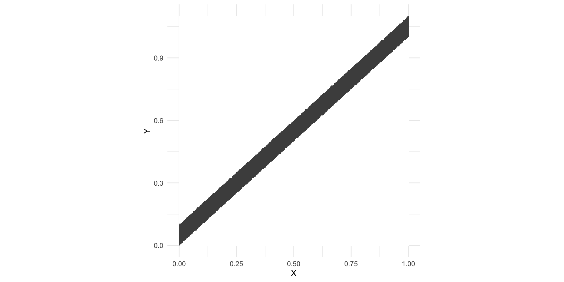
Example 1

In gray: the region where f_{X,Y}(x,y)>0

• When X increases, Y increases linearly (not surprising, since Y = X + Z)
• We expect the correlation \rho_{XY} to be close to 1

Example 1 – Computing \rho_{XY}

• For a random variable W \sim {\rm uniform} (a,b), we have {\rm I\kern-.3em E}[W] = \frac{a+b}{2} \,, \qquad {\rm Var}[W] = \frac{(b-a)^2}{12}

• Since X \sim {\rm uniform} (0,1) and Z \sim {\rm uniform} (0,1/10), we have {\rm I\kern-.3em E}[X] = \frac12 \,, \qquad {\rm Var}[X] = \frac{1}{12} \,, \qquad {\rm I\kern-.3em E}[Z] = \frac{1}{20} \,, \qquad {\rm Var}[Z] = \frac{1}{1200}

• Since X and Z are independent, we also have {\rm Var}[Y] = {\rm Var}[X + Z] = {\rm Var}[X] + {\rm Var}[Z] = \frac{1}{12} + \frac{1}{1200}

Example 1 – Computing \rho_{XY}

• Since X and Z are independent, we have {\rm I\kern-.3em E}[XZ] = {\rm I\kern-.3em E}[X]{\rm I\kern-.3em E}[Z]

• We conclude that \begin{align*} {\rm Cov}(X,Y) & = {\rm I\kern-.3em E}[XY] - {\rm I\kern-.3em E}[X] {\rm I\kern-.3em E}[Y] \\ & = {\rm I\kern-.3em E}[X(X + Z)] - {\rm I\kern-.3em E}[X] {\rm I\kern-.3em E}[X + Z] \\ & = {\rm I\kern-.3em E}[X^2] - {\rm I\kern-.3em E}[X]^2 + {\rm I\kern-.3em E}[XZ] - {\rm I\kern-.3em E}[X]{\rm I\kern-.3em E}[Z] \\ & = {\rm Var}[X] = \frac{1}{12} \end{align*}

Example 1 – Computing \rho_{XY}

• The correlation between X and Y is \begin{align*} \rho_{XY} & = \frac{{\rm Cov}(X,Y)}{\sqrt{{\rm Var}[X]}\sqrt{{\rm Var}[Y]}} \\ & = \frac{\frac{1}{12}}{\sqrt{\frac{1}{12}} \sqrt{ \frac{1}{12} + \frac{1}{1200}} } = \sqrt{\frac{100}{101}} \end{align*}

• As expected, we have very high correlation \rho_{XY} \approx 1

• This confirms a very strong linear relationship between X and Y

Example 2

• Assume X and Z are independent, and X \sim {\rm uniform} \left( -1,1 \right) \,, \qquad Z \sim {\rm uniform} \left( 0, \frac{1}{10} \right)

• Define the random variable Y = X^2 + Z

• Since X and Z are independent, and Z is uniform, we have that Y | X = x \, \sim \, {\rm uniform} \left( x^2, x^2 + \frac{1}{10} \right) (adding x^2 to Z simply shifts the uniform distribution of Z by x^2)

• Question: Is the correlation \rho_{XY} between X and Y high or low?

Example 2

• As Y | X \, \sim \, {\rm uniform} \left( X^2, X^2 + \frac{1}{10} \right), the conditional pdf of Y given X = x is f(y|x) = \begin{cases} 10 & \text{ if } \, y \in \left( x^2 , x^2 + \frac{1}{10} \right) \\ 0 & \text{ otherwise} \end{cases}

• As X \sim {\rm uniform} (-1,1), its pdf is f_X(x) = \begin{cases} \frac12 & \text{ if } \, x \in \left( -1 , 1 \right) \\ 0 & \text{ otherwise} \end{cases}

• Therefore, the joint distribution of (X,Y) is f_{X,Y}(x,y) = f(y|x)f_X(x) = \begin{cases} 10 & \text{ if } \, x \in (-1,1) \, \text{ and } \, y \in \left( x^2 , x^2 + \frac{1}{10} \right) \\ 0 & \text{ otherwise} \end{cases}

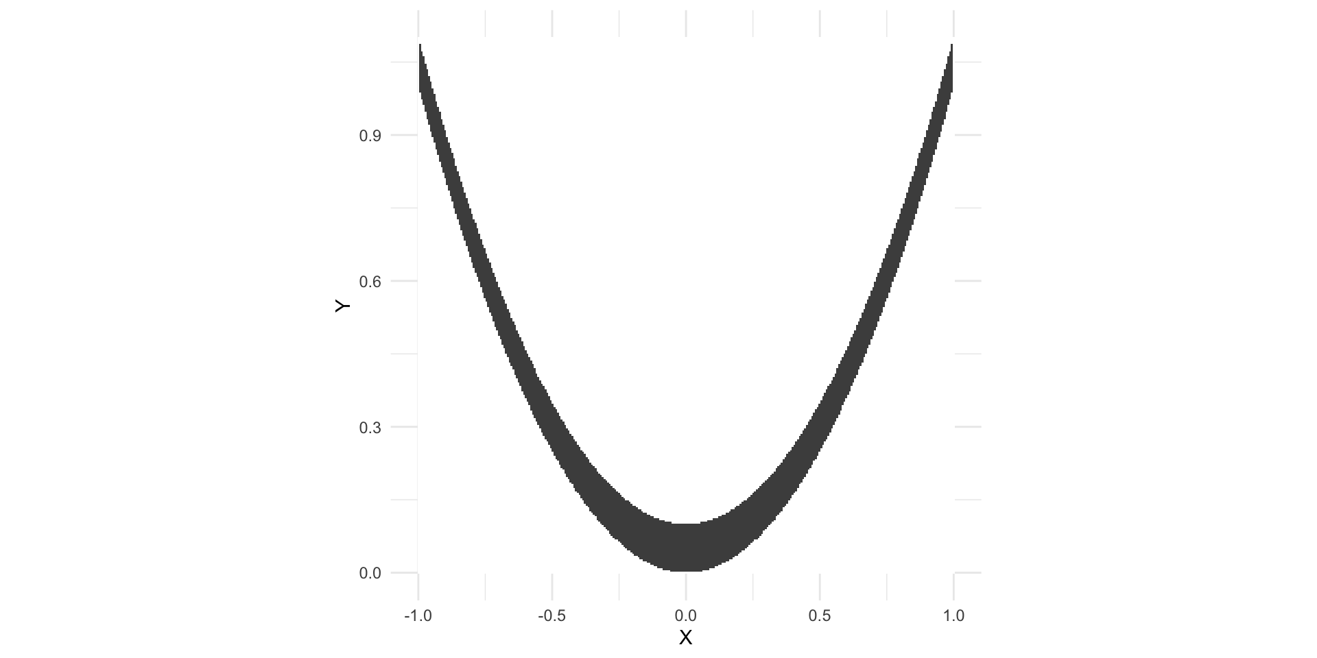
Example 2

In gray: the region where f_{X,Y}(x,y)>0

• When X increases, Y increases quadratically (not surprising, as Y = X^2 + Z)
• There is no linear relationship between X and Y \,\, \implies \,\, we expect \, \rho_{XY} \approx 0

Example 2 – Computing \rho_{XY}

• Since X \sim {\rm uniform} (-1,1), we can compute that {\rm I\kern-.3em E}[X] = {\rm I\kern-.3em E}[X^3] = 0

• Since X and Z are independent, we have {\rm I\kern-.3em E}[XZ] = {\rm I\kern-.3em E}[X]{\rm I\kern-.3em E}[Z] = 0

Example 2 – Computing \rho_{XY}

• Compute the covariance \begin{align*} {\rm Cov}(X,Y) & = {\rm I\kern-.3em E}[XY] - {\rm I\kern-.3em E}[X] {\rm I\kern-.3em E}[Y] \\ & = {\rm I\kern-.3em E}[XY] \\ & = {\rm I\kern-.3em E}[X(X^2 + Z)] \\ & = {\rm I\kern-.3em E}[X^3] + {\rm I\kern-.3em E}[XZ] = 0 \end{align*}

• The correlation between X and Y is \rho_{XY} = \frac{{\rm Cov}(X,Y)}{\sqrt{{\rm Var}[X]}\sqrt{{\rm Var}[Y]}} = 0

• This confirms there is no linear relationship between X and Y

Part 2:
Multivariate random vectors

Multivariate Random Vectors

Recall

• A Random vector is a function \mathbf{X}\colon \Omega \to \mathbb{R}^n
• \mathbf{X} is a multivariate random vector if n \geq 3
• We denote the components of \mathbf{X} by \mathbf{X}= (X_1,\ldots,X_n) \,, \qquad X_i \colon \Omega \to \mathbb{R}
• We denote the components of a point \mathbf{x}\in \mathbb{R}^n by \mathbf{x}= (x_1,\ldots,x_n)

Discrete and Continuous Multivariate Random Vectors

Everything we defined for bivariate vectors extends to multivariate vectors

Definition

The random vector \mathbf{X}\colon \Omega \to \mathbb{R}^n is:

• continuous if components X_is are continuous
• discrete if components X_i are discrete

Joint pmf

Definition

The joint pmf of a continuous random vector \mathbf{X} is f_{\mathbf{X}} \colon \mathbb{R}^n \to \mathbb{R} defined by f_{\mathbf{X}} (\mathbf{x}) = f_{\mathbf{X}}(x_1,\ldots,x_n) := P(X_1 = x_1 , \ldots , X_n = x_n ) \,, \qquad \forall \, \mathbf{x}\in \mathbb{R}^n

Note: For all A \subset \mathbb{R}^n it holds P(\mathbf{X}\in A) = \sum_{\mathbf{x}\in A} f_{\mathbf{X}}(\mathbf{x})

Joint pdf

Definition

The joint pdf of a continuous random vector \mathbf{X} is a function f_{\mathbf{X}} \colon \mathbb{R}^n \to \mathbb{R} such that P (\mathbf{X}\in A) := \int_A f_{\mathbf{X}}(x_1 ,\ldots, x_n) \, dx_1 \ldots dx_n = \int_{A} f_{\mathbf{X}}(\mathbf{x}) \, d\mathbf{x}\,, \quad \forall \, A \subset \mathbb{R}^n

Note: \int_A denotes an n-fold intergral over all points \mathbf{x}\in A

Expected Value

Definition

\mathbf{X}\colon \Omega \to \mathbb{R}^n random vector and g \colon \mathbb{R}^n \to \mathbb{R} function. The expected value of the random variable g(X) is \begin{align*} {\rm I\kern-.3em E}[g(\mathbf{X})] & := \sum_{x \in \mathbb{R}^n} g(\mathbf{x}) f_{\mathbf{X}} (\mathbf{x}) \qquad & (\mathbf{X}\text{ discrete}) \\ {\rm I\kern-.3em E}[g(\mathbf{X})] & := \int_{\mathbb{R}^n} g(\mathbf{x}) f_{\mathbf{X}} (\mathbf{x}) \, d\mathbf{x}\qquad & \qquad (\mathbf{X}\text{ continuous}) \end{align*}

Marginal distributions

• Marginal pmf or pdf of any subset of the coordinates (X_1,\ldots,X_n) can be computed by integrating or summing the remaining coordinates

• To ease notations, we only define maginals wrt the first k coordinates

Definition

The marginal pmf or marginal pdf of the random vector \mathbf{X} with respect to the first k coordinates is the function f \colon \mathbb{R}^k \to \mathbb{R} defined by \begin{align*} f(x_1,\ldots,x_k) & := \sum_{ (x_{k+1}, \ldots, x_n) \in \mathbb{R}^{n-k} } f_{\mathbf{X}} (x_1 , \ldots , x_n) \quad & (\mathbf{X}\text{ discrete}) \\ f(x_1,\ldots,x_k) & := \int_{\mathbb{R}^{n-k}}f_{\mathbf{X}} (x_1 , \ldots, x_n ) \, dx_{k+1} \ldots dx_{n} \quad & \quad (\mathbf{X}\text{ continuous}) \end{align*}

Marginal distributions

We use a special notation for marginal pmf or pdf wrt a single coordinate

Definition

The marginal pmf or pdf of the random vector \mathbf{X} with respect to the i-th coordinate is the function f_{X_i} \colon \mathbb{R}\to \mathbb{R} defined by \begin{align*} f_{X_i}(x_i) & := \sum_{ \tilde{x} \in \mathbb{R}^{n-1} } f_{\mathbf{X}} (x_1, \ldots, x_n) \quad & (\mathbf{X}\text{ discrete}) \\ f_{X_i}(x_i) & := \int_{\mathbb{R}^{n-1}}f_{\mathbf{X}} (x_1, \ldots, x_n) \, d\tilde{x} \quad & \quad (\mathbf{X}\text{ continuous}) \end{align*} where \tilde{x} \in \mathbb{R}^{n-1} denotes the vector \mathbf{x} with i-th component removed \tilde{x} := (x_1, \ldots, x_{i-1}, x_{i+1},\ldots, x_n)

Conditional distributions

We now define conditional distributions given the first k coordinates

Definition

Let \mathbf{X} be a random vector and suppose that the marginal pmf or pdf wrt the first k coordinates satisfies f(x_1,\ldots,x_k) > 0 \,, \quad \forall \, (x_1,\ldots,x_k ) \in \mathbb{R}^k The conditional pmf or pdf of (X_{k+1},\ldots,X_n) given X_1 = x_1, \ldots , X_k = x_k is the function of (x_{k+1},\ldots,x_{n}) defined by f(x_{k+1},\ldots,x_n | x_1 , \ldots , x_k) := \frac{f_{\mathbf{X}}(x_1,\ldots,x_n)}{f(x_1,\ldots,x_k)}

Conditional distributions

Similarly, we can define the conditional distribution given the i-th coordinate

Definition

Let \mathbf{X} be a random vector and suppose that for a given x_i \in \mathbb{R} f_{X_i}(x_i) > 0 The conditional pmf or pdf of \tilde{X} given X_i = x_i is the function of \tilde{x} defined by f(\tilde{x} | x_i ) := \frac{f_{\mathbf{X}}(x_1,\ldots,x_n)}{f_{X_i}(x_i)} where we denote \tilde{X} := (X_1, \ldots, X_{i-1}, X_{i+1},\ldots, X_n) \,, \quad \tilde{x} := (x_1, \ldots, x_{i-1}, x_{i+1},\ldots, x_n)

Independence

Definition

\mathbf{X}=(X_1,\ldots,X_n) random vector with joint pmf or pdf f_{\mathbf{X}} and marginals f_{X_i}. We say that the random variables X_1,\ldots,X_n are mutually independent if f_{\mathbf{X}}(x_1,\ldots,x_n) = f_{X_1}(x_1) \cdot \ldots \cdot f_{X_n}(x_n) = \prod_{i=1}^n f_{X_i}(x_i)

Proposition

If X_1,\ldots,X_n are mutually independent then for all A_i \subset \mathbb{R} P(X_1 \in A_1 , \ldots , X_n \in A_n) = \prod_{i=1}^n P(X_i \in A_i)

Independence

Characterization result

Theorem

\mathbf{X}=(X_1,\ldots,X_n) random vector with joint pmf or pdf f_{\mathbf{X}}. They are equivalent:

• The random variables X_1,\ldots,X_n are mutually independent
• There exist functions g_i(x_i) such that f_{\mathbf{X}}(x_1,\ldots,x_n) = \prod_{i=1}^n g_{i}(x_i)

Independence

A very useful theorem

Theorem

Let X_1,\ldots,X_n be mutually independent random variables and g_i(x_i) function only of x_i. Then the random variables g_1(X_1) \,, \ldots \,, g_n(X_n) are mutually independent

Proof: Omitted. See [1] page 184

Example: X_1,\ldots,X_n \, independent \,\, \implies \,\, X_1^2, \ldots, X_n^2 \, independent

Independence

Expectation of product

Theorem

Let X_1,\ldots,X_n be mutually independent random variables and g_i(x_i) functions. Then {\rm I\kern-.3em E}[ g_1(X_1) \cdot \ldots \cdot g_n(X_n) ] = \prod_{i=1}^n {\rm I\kern-.3em E}[g_i(X_i)]

Application: MGF of sums

Theorem

Let X_1,\ldots,X_n be mutually independent random variables, with mgfs M_{X_1}(t),\ldots, M_{X_n}(t). Define the random variable Z := X_1 + \ldots + X_n The mgf of Z satisfies M_Z(t) = \prod_{i=1}^n M_{X_i}(t)

Application: MGF of sums

Proof of Theorem

Follows by the previous Theorem

\begin{align*} M_{Z} (t) & = {\rm I\kern-.3em E}[e^{tZ}] \\ & = {\rm I\kern-.3em E}[\exp( t X_1 + \ldots + tX_n)] \\ & = {\rm I\kern-.3em E}\left[ e^{t X_1} \cdot \ldots \cdot e^{ t X_n} \right] \\ & = \prod_{i=1}^n {\rm I\kern-.3em E}[e^{tX_i}] \\ & = \prod_{i=1}^n M_{X_i}(t) \end{align*}

Example – Sum of independent Normals

Theorem

Let X_1,\ldots,X_n be mutually independent random variables with normal distribution X_i \sim N (\mu_i,\sigma_i^2). Define Z := X_1 + \ldots + X_n and \mu :=\mu_1 + \ldots + \mu_n \,, \quad \sigma^2 := \sigma_1^2 + \ldots + \sigma_n^2 Then Z is normally distributed with Z \sim N(\mu,\sigma^2)

Example – Sum of independent Normals

Proof of Theorem

• We have seen in Lecture 1 that X_i \sim N(\mu_i,\sigma_i^2) \quad \implies \quad M_{X_i}(t) = \exp \left( \mu_i t + \frac{t^2 \sigma_i^2}{2} \right)

• As X_1,\ldots,X_n are mutually independent, from the Theorem in Slide 47, we get \begin{align*} M_{Z}(t) & = \prod_{i=1}^n M_{X_i}(t) = \prod_{i=1}^n \exp \left( \mu_i t + \frac{t^2 \sigma_i^2}{2} \right) \\ & = \exp \left( (\mu_1 + \ldots + \mu_n) t + \frac{t^2 (\sigma_1^2 + \ldots +\sigma_n^2)}{2} \right) \\ & = \exp \left( \mu t + \frac{t^2 \sigma^2 }{2} \right) \end{align*}

Example – Sum of independent Normals

Proof of Theorem

• Therefore Z has moment generating function M_{Z}(t) = \exp \left( \mu t + \frac{t^2 \sigma^2 }{2} \right)

• The above is the mgf of a normal distribution with \text{mean }\quad \mu \quad \text{ and variance} \quad \sigma^2

• Since mgfs characterize distributions (see Theorem in Slide 71 of Lecture 1), we conclude Z \sim N(\mu, \sigma^2 )

Example – Sum of independent Gammas

Theorem

Let X_1,\ldots,X_n be mutually independent random variables with Gamma distribution X_i \sim \Gamma (\alpha_i,\beta). Define Z := X_1 + \ldots + X_n and \alpha :=\alpha_1 + \ldots + \alpha_n Then Z has Gamma distribution Z \sim \Gamma(\alpha,\beta)

Example – Sum of independent Gammas

Proof of Theorem

• We have seen in Lecture 1 that X_i \sim \Gamma(\alpha_i,\beta) \qquad \implies \qquad M_{X_i}(t) = \frac{\beta^{\alpha_i}}{(\beta-t)^{\alpha_i}}

• As X_1,\ldots,X_n are mutually independent, from the Theorem in Slide 47, we get \begin{align*} M_{Z}(t) & = \prod_{i=1}^n M_{X_i}(t) = \prod_{i=1}^n \frac{\beta^{\alpha_i}}{(\beta-t)^{\alpha_i}} \\ & = \frac{\beta^{(\alpha_1 + \ldots + \alpha_n)}}{(\beta-t)^{(\alpha_1 + \ldots + \alpha_n)}} \\ & = \frac{\beta^{\alpha}}{(\beta-t)^{\alpha}} \end{align*}

Example – Sum of independent Gammas

Proof of Theorem

• Therefore Z has moment generating function M_{Z}(t) = \frac{\beta^{\alpha}}{(\beta-t)^{\alpha}}

• The above is the mgf of a Gamma distribution with parameters \alpha and \beta

• Since mgfs characterize distributions (see Theorem in Slide 71 of Lecture 1), we conclude Z \sim \Gamma(\alpha, \beta )

Expectation of sums

Expectation is linear

Theorem

For random variables X_1,\ldots,X_n and scalars a_1,\ldots,a_n we have {\rm I\kern-.3em E}[a_1X_1 + \ldots + a_nX_n] = a_1 {\rm I\kern-.3em E}[X_1] + \ldots + a_n {\rm I\kern-.3em E}[X_n]

Variance of sums

Variance is quadratic

Theorem

For random variables X_1,\ldots,X_n and scalars a_1,\ldots,a_n we have \begin{align*} {\rm Var}[a_1X_1 + \ldots + a_nX_n] = a_1^2 {\rm Var}[X_1] & + \ldots + a^2_n {\rm Var}[X_n] \\ & + 2 \sum_{i \neq j} {\rm Cov}(X_i,X_j) \end{align*} If X_1,\ldots,X_n are mutually independent then {\rm Var}[a_1X_1 + \ldots + a_nX_n] = a_1^2 {\rm Var}[X_1] + \ldots + a^2_n {\rm Var}[X_n]

Part 3:
Random samples

iid random variables

Definition

The random variables X_1,\ldots,X_n are independent identically distributed or iid with pdf or pmf f(x) if

• X_1,\ldots,X_n are mutually independent
• The marginal pdf or pmf of each X_i satisfies f_{X_i}(x) = f(x) \,, \quad \forall \, x \in \mathbb{R}

Random sample

• Suppose the data in an experiment consists of observations on a population
• Suppose the population has distribution f(x)
• Each observation is labelled X_i
• We always assume that the population is infinite
• Therefore each X_i has distribution f(x)
• We also assume the observations are independent

Definition

The random variables X_1,\ldots,X_n are a random sample of size n from the population f(x) if X_1,\ldots,X_n are iid with pdf or pmf f(x)

Random sample

Remark: Let X_1,\ldots,X_n be a random sample of size n from the population f(x). The joint distribution of \mathbf{X}= (X_1,\ldots,X_n) is f_{\mathbf{X}}(x_1,\ldots,x_n) = f(x_1) \cdot \ldots \cdot f(x_n) = \prod_{i=1}^n f(x_i) (since the X_is are mutually independent with distribution f)

Definition

We call f_{\mathbf{X}} the joint sample distribution

Random sample

Notation:

• When the population distribution f(x) depends on a parameter \theta we write f = f(x|\theta)

• In this case the joint sample distribution is f_{\mathbf{X}}(x_1,\ldots,x_n | \theta) = \prod_{i=1}^n f(x_i | \theta)

Example

• Suppose a population has \mathop{\mathrm{Exponential}}(\beta) distribution f(x|\beta) = \frac{1}{\beta} e^{-x/\beta} \,, \qquad \text{ if } \,\, x > 0
• Suppose X_1,\ldots,X_n is random sample from the population f(x|\beta)
• The joint sample distribution is then \begin{align*} f_{\mathbf{X}}(x_1,\ldots,x_n | \beta) & = \prod_{i=1}^n f(x_i|\beta) \\ & = \prod_{i=1}^n \frac{1}{\beta} e^{-x_i/\beta} \\ & = \frac{1}{\beta^n} e^{-(x_1 + \ldots + x_n)/\beta} \end{align*}

Example

• We have P(X_1 > 2) = \int_{2}^\infty f(x|\beta) \, dx = \int_{2}^\infty \frac{1}{\beta} e^{-x/\beta} \, dx = e^{-2/\beta}

• Thanks to iid assumption we can easily compute \begin{align*} P(X_1 > 2 , \ldots, X_n > 2) & = \prod_{i=1}^n P(X_i > 2) \\ & = \prod_{i=1}^n P(X_1 > 2) \\ & = P(X_1 > 2)^n \\ & = e^{-2n/\beta} \end{align*}

Part 4:
Unbiased estimators

Point estimation

Usual situation: Suppose a population has distribution f(x|\theta)

• In general, the parameter \theta is unknown
• Suppose that knowing \theta is sufficient to characterize f(x|\theta)

Example: A population could be normally distributed f(x|\mu,\sigma^2) = \frac{1}{\sqrt{2\pi\sigma}} \, \exp\left( -\frac{(x-\mu)^2}{2\sigma^2}\right) \,, \quad x \in \mathbb{R}

• Here \mu is the mean and \sigma^2 the variance
• Knowing \mu and \sigma^2 completely characterizes the normal distribution

Point estimation

Goal: We want to make predictions about the population

• In order to do that, we need to know the population distribution f(x|\theta)

• It is therefore desirable to determine \theta, with reasonable certainty

Definitions:

• Point estimation is the procedure of estimating \theta from random sample

• A point estimator is any function of a random sample W(X_1,\ldots,X_n)

• Point estimators are also called statistics

Unbiased estimator

Definition

Suppose W is a point estimator of a parameter \theta

• The bias of W is the quantity \rm{Bias}_{\theta} := {\rm I\kern-.3em E}[W] - \theta

• W is an unbiased estimator if \rm{Bias}_{\theta} = 0, that is, {\rm I\kern-.3em E}[W] = \theta

Note: A point estimator W = W(X_1, \ldots, X_n) is itself a random variable. Thus {\rm I\kern-.3em E}[W] is the mean of such random variable

Next goal

• We want to estimate mean and variance of a population

• Unbiased estimators for such quantities are:

  • Sample mean
  • Sample variance

Estimating the population mean

Problem

Suppose to have a population with distribution f(x|\theta) We want to estimate the population mean \mu := \int_{\mathbb{R}} x f(x|\theta) \, dx

Sample mean

Definition

The sample mean of a random sample X_1,\ldots,X_n is the statistic W(X_1,\ldots,X_n) := \overline{X} := \frac{1}{n} \sum_{i=1}^n X_i

Sample mean

Sample mean is unbiased estimator of mean

Theorem

The sample mean \overline{X} is an unbiased estimator of the population mean \mu, that is, {\rm I\kern-.3em E}[\overline{X}] = \mu

Sample mean

Proof of theorem

• X_1,\ldots,X_n is a random sample from f(x|\theta)

• Therefore X_i \sim f(x|\theta) and {\rm I\kern-.3em E}[X_i] = \int_{\mathbb{R}} x f(x|\theta) \, dx = \mu

• By linearity of expectation we have {\rm I\kern-.3em E}[\overline{X}] = \frac{1}{n} \sum_{i=1}^n {\rm I\kern-.3em E}[X_i] = \frac{1}{n} \sum_{i=1}^n \mu = \mu

• This shows \overline{X} is an unbiased estimator of \mu

Variance of Sample mean

For reasons clear later, it is useful to compute the variance of the sample mean \overline{X}

Lemma

X_1,\ldots,X_n random sample from population with mean \mu and variance \sigma^2. Then {\rm Var}[\overline{X}] = \frac{\sigma^2}{n}

Variance of Sample mean

Proof of Lemma

• By assumption,the population has mean \mu and variance \sigma^2

• Since X_i is sampled from the population, we have {\rm I\kern-.3em E}[X_i] = \mu \,, \quad {\rm Var}[X_i] = \sigma^2

• Since the variance is quadratic, and the X_is are independent, \begin{align*} {\rm Var}[\overline{X}] & = {\rm Var}\left[ \frac{1}{n} \sum_{i=1}^n X_i \right] = \frac{1}{n^2} \sum_{i=1}^n {\rm Var}[X_i] \\ & = \frac{1}{n^2} \cdot n \sigma^2 = \frac{\sigma^2}{n} \end{align*}

Estimating the population variance

Problem

Suppose to have a population f(x|\theta) with mean \mu and variance \sigma^2. We want to estimate the population variance

Sample variance

Definition

The sample variance of a random sample X_1,\ldots,X_n is the statistic S^2 := \frac{1}{n-1} \sum_{i=1}^n \left( X_i - \overline{X} \right)^2 where \overline{X} is the sample mean \overline{X} := \frac{1}{n} \sum_{i=1}^n X_i

Sample variance

Equivalent formulation

Proposition

It holds that S^2 := \frac{ \sum_{i=1}^n \left( X_i - \overline{X} \right)^2}{n-1} = \frac{ \sum_{i=1}^n X_i^2 - n\overline{X}^2 }{n-1}

Sample variance

Proof of Proposition

• We have \begin{align*} \sum_{i=1}^n \left( X_i - \overline{X} \right)^2 & = \sum_{i=1}^n \left(X_i^2 + \overline{X}^2 - 2 X_i \overline{X} \right) = \sum_{i=1}^n X_i^2 + n\overline{X}^2 - 2 \overline{X} \sum_{i=1}^n X_i \\ & = \sum_{i=1}^n X_i^2 + n\overline{X}^2 - 2 n \overline{X}^2 = \sum_{i=1}^n X_i^2 -n \overline{X}^2 \end{align*}

• Dividing by n-1 yields the desired identity S^2 = \frac{ \sum_{i=1}^n X_i^2 -n \overline{X}^2 }{n-1}

Sample variance

Sample variance is unbiased estimator of variance

Theorem

The sample variance S^2 is an unbiased estimator of the population variance \sigma^2, that is, {\rm I\kern-.3em E}[S^2] = \sigma^2

Sample variance

Proof of theorem

• By linearity of expectation we infer {\rm I\kern-.3em E}[(n-1)S^2] = {\rm I\kern-.3em E}\left[ \sum_{i=1}^n X_i^2 - n\overline{X}^2 \right] = \sum_{i=1}^n {\rm I\kern-.3em E}[X_i^2] - n {\rm I\kern-.3em E}[\overline{X}^2]

• Since X_i \sim f(x|\theta), we have {\rm I\kern-.3em E}[X_i] = \mu \,, \quad {\rm Var}[X_i] = \sigma^2

• Therefore by definition of variance, we infer {\rm I\kern-.3em E}[X_i^2] = {\rm Var}[X_i] + {\rm I\kern-.3em E}[X]^2 = \sigma^2 + \mu^2

Sample variance

Proof of theorem

• Also recall that {\rm I\kern-.3em E}[\overline{X}] = \mu \,, \quad {\rm Var}[\overline{X}] = \frac{\sigma^2}{n}

• By definition of variance, we get {\rm I\kern-.3em E}[\overline{X}^2] = {\rm Var}[\overline{X}] + {\rm I\kern-.3em E}[\overline{X}]^2 = \frac{\sigma^2}{n} + \mu^2

Sample variance

Proof of theorem

• Hence \begin{align*} {\rm I\kern-.3em E}[(n-1)S^2] & = \sum_{i=1}^n {\rm I\kern-.3em E}[X_i^2] - n {\rm I\kern-.3em E}[\overline{X}^2] \\ & = \sum_{i=1}^n \left( \mu^2 + \sigma^2 \right) - n \left( \mu^2 + \frac{\sigma^2}{n} \right) \\ & = n\mu^2 + n\sigma^2 - n \mu^2 - \sigma^2 \\ & = (n-1) \sigma^2 \end{align*}

• Dividing both sides by (n-1) yields the thesis {\rm I\kern-.3em E}[S^2] = \sigma^2

Additional note

• The sample variance is defined by S^2=\frac{\sum_{i=1}^{n} (X_i-\overline{X})^2}{n-1}=\frac{\sum_{i=1}^n X_i^2-n{\overline{X}^2}}{n-1}

• Where does the n-1 factor in the denominator come from?
  (It would look more natural to divide by n, instead that by n-1)

• The n-1 factor is caused by a loss of precision:

  • Ideally, the sample variance S^2 should contain the population mean \mu
  • Since \mu is not available, we estimate it with the sample mean \overline{X}
  • This leads to the loss of 1 degree of freedom

Additional note

• General statistical rule: \text{Lose 1 degree of freedom for each parameter estimated}

• In the case of the sample variance S^2, we have to estimate one parameter (the population mean \mu). Hence \begin{align*} \text{degrees of freedom} & = \text{Sample size}-\text{No. of estimated parameters} \\ & = n-1 \end{align*}

• This is where the n-1 factor comes from!

Notation

• The realization of a random sample X_1,\ldots,X_n is denoted by x_1, \ldots, x_n

• The realization of the sample mean \overline{X} is denoted \overline{x} := \frac{1}{n} \sum_{i=1}^n x_i

• The realization of the sample variance S^2 is denoted s^2=\frac{\sum_{i=1}^{n}(x_i-\overline{x})^2}{n-1}=\frac{\sum_{i=1}^n x_i^2-n{\overline{x}^2}}{n-1}

• Capital letters denote random variables, while lowercase letters denote specific values (realizations) of those variables

Exercise

Wage data on 10 Mathematicians

Mathematician	x_1	x_2	x_3	x_4	x_5	x_6	x_7	x_8	x_9	x_{10}
Wage	36	40	46	54	57	58	59	60	62	63

Question: Estimate population mean and variance

Solution to the Exercise

• Number of advertising professionals n=10

• Sample Mean: \overline{x} = \frac{1}{n} \sum_{i=1}^n x_i = \frac{36+40+46+{\dots}+62+63}{10}=\frac{535}{10}=53.5

• Sample Variance: \begin{align*} s^2 & = \frac{\sum_{i=1}^n x_{i}^2 - n \overline{x}^2}{n-1} \\ \sum_{i=1}^n x_i^2 & = 36^2+40^2+46^2+{\ldots}+62^2+63^2 = 29435 \\ s^2 & = \frac{29435-10(53.5)^2}{9} = 90.2778 \end{align*}

Part 5:
Chi-squared distribution

Overview

Chi-squared distribution:

• defined in terms of squares of N(0, 1) random variables
• designed to describe variance estimation
• used to define other members of the normal family
  • Student t-distribution
  • F-distribution

Why the normal family is important

• Classical hypothesis testing and regression problems
• The same maths solves apparently unrelated problems
• Easy to compute
  • Statistics tables
  • Software
• Enables the development of approximate methods in more complex (and interesting) problems

Reminder: Normal distribution

• X has normal distribution with mean \mu and variance \sigma^2 if pdf is f(x) := \frac{1}{\sqrt{2\pi\sigma^2}} \, \exp\left( -\frac{(x-\mu)^2}{2\sigma^2}\right) \,, \quad x \in \mathbb{R}

• In this case we write X \sim N(\mu,\sigma^2)

• The standard normal distribution is denoted N(0,1)

Chi-squared distribution

Definition

Definition

Let Z_1,\ldots,Z_r be iid N(0, 1) random variables. The chi-squared distribution with r degrees of freedom is the distribution \chi^2_r \sim Z^2_1+...+Z^2_r

Chi-squared distribution

Pdf characterization

Theorem

The \chi^2_r distribution is equivalent to a Gamma distribution \chi^2_r \sim \Gamma(r/2, 1/2) Therefore the pdf of \chi^2_r can be written in closed form as f_{\chi^2_r}(x)=\frac{x^{(r/2)-1} \, e^{-x/2}}{\Gamma(r/2) 2^{r/2}} \,, \quad x>0

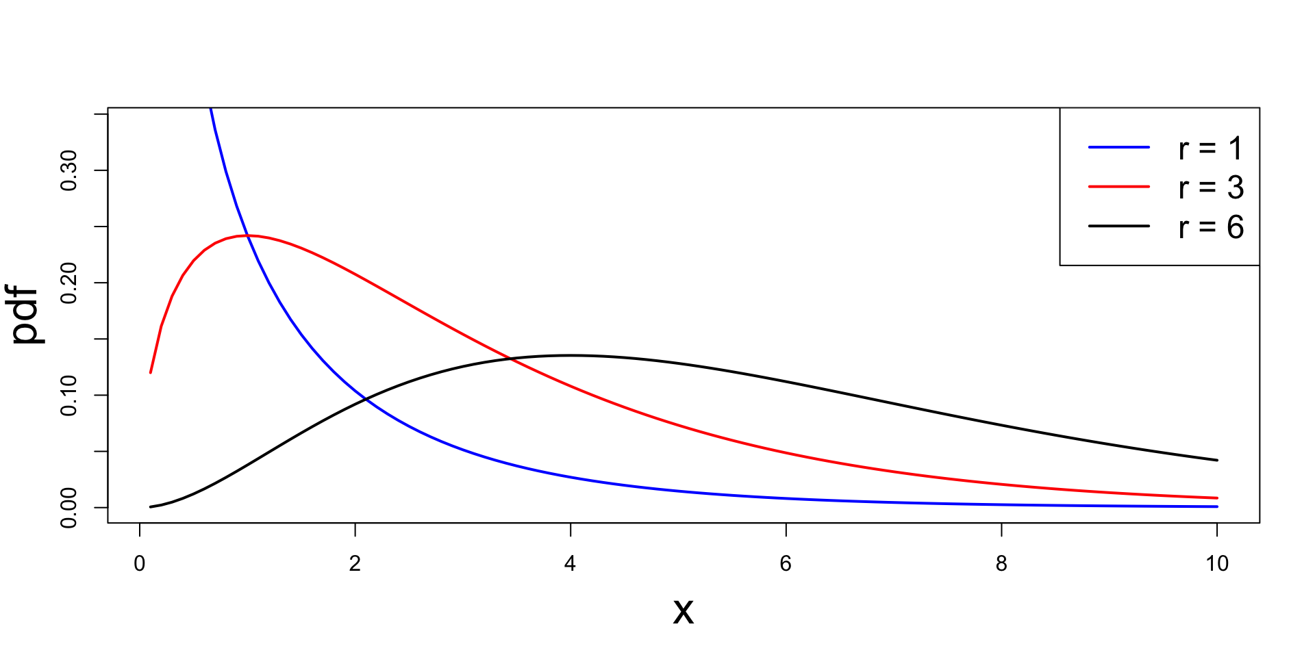
Chi-squared distribution

Plots of chi-squared pdf for different choices of r

Proof of Theorem – Case r =1

• We start with the case r=1
• Need to prove that \chi^2_1 \sim \Gamma(1/2, 1/2)
• Therefore we need to show that the pdf of \chi^2_1 is f_{\chi^2_1}(x)=\frac{x^{-1/2} \, e^{-x/2}}{\Gamma(1/2) 2^{1/2}} \,, \quad x>0

Proof of Theorem – Case r =1

• To this end, notice that by definition \chi^2_1 \sim Z^2 \,, \qquad Z \sim N(0,1)
• Hence, for x>0 we can compute cdf via \begin{align*} F_{\chi^2_1}(x) & = P(\chi^2_1 \leq x) \\ & = P(Z^2 \leq x ) \\ & = P(- \sqrt{x} \leq Z \leq \sqrt{x} ) \\ & = 2 P (0 \leq Z \leq \sqrt{x}) \end{align*} where in the last equality we used symmetry of Z around x=0

Proof of Theorem – Case r =1

• Recalling the definition of standard normal pdf we get \begin{align*} F_{\chi^2_1}(x) & = 2 P (0 \leq Z \leq \sqrt{x}) \\ & = 2 \frac{1}{\sqrt{2\pi}} \int_0^{\sqrt{x}} e^{-t^2/2} \, dt \\ & = 2 \frac{1}{\sqrt{2\pi}} G( \sqrt{x} ) \end{align*} where we set G(x) := \int_0^{x} e^{-t^2/2} \, dt

Proof of Theorem – Case r =1

• We can now compute pdf of \chi_1^2 by differentiating the cdf

• By the Fundamental Theorem of Calculus we have G'(x) = \frac{d}{dx} \left( \int_0^{x} e^{-t^2/2} \, dt \right) = e^{-x^2/2} \quad \implies \quad G'(\sqrt{x}) = e^{-x/2}

• Chain rule yields \begin{align*} f_{\chi^2_1}(x) & = \frac{d}{dx} F_{\chi^2_1}(x) = \frac{d}{dx} \left( 2 \frac{1}{\sqrt{2\pi}} G( \sqrt{x} ) \right) \\ & = 2 \frac{1}{\sqrt{2\pi}} G'( \sqrt{x} ) \frac{x^{-1/2}}{2} = \frac{x^{-1/2} e^{-x/2}}{2^{1/2} \sqrt{\pi}} \end{align*}

Proof of Theorem – Case r =1

• It is well known that \Gamma(1/2) = \sqrt{\pi}
• Hence, we conclude f_{\chi^2_1}(x) = \frac{x^{-1/2} e^{-x/2}}{2^{1/2} \sqrt{\pi}} = \frac{x^{-1/2} e^{-x/2}}{2^{1/2} \Gamma(1/2)}
• This shows \chi_1^2 \sim \Gamma(1/2,1/2)

Proof of Theorem – Case r \geq 2

• We need to prove that \chi^2_r \sim \Gamma(r/2, 1/2)

• By definition \chi^2_r \sim Z^2_1 + \ldots + Z^2_r \,, \qquad Z_i \sim N(0,1) \quad \text{iid}

• By the Theorem in Slide 46, we have Z_1,\ldots,Z_r \,\,\, \text{iid} \quad \implies \quad Z_1^2,\ldots,Z_r^2 \,\,\, \text{iid}

• Moreover, by definition, Z_i^2 \sim \chi_1^2

• Therefore, we have \chi^2_r = \sum_{i=1}^r X_i, \qquad X_i \sim \chi^2_1 \quad \text{iid}

Proof of Theorem – Case r \geq 2

• We have just proven that \chi_1^2 \sim \Gamma (1/2,1/2)

• Moreover, the Theorem in Slide 53 guarantees that Y_i \sim \Gamma(\alpha_i, \beta) \quad \text{independent} \quad \implies \quad Y_1 + \ldots + Y_n \sim \Gamma(\alpha,\beta) where \alpha = \alpha_1 + \ldots + \alpha_n

• Therefore, we conclude that \chi^2_r = \sum_{i=1}^r X_i, \qquad X_i \sim \Gamma(1/2,1/2) \quad \text{iid} \quad \implies \quad \chi^2_r \sim \Gamma(r/2,1/2)

Part 6:
Sampling from normal distribution

Sampling from Normal distribution

Sample mean and variance: For a random sample X_1,\ldots,X_n defined by S^2 := \frac{1}{n-1} \sum_{i=1}^n \left( X_i - \overline{X} \right)^2 \,, \qquad \overline{X} := \frac{1}{n} \sum_{i=1}^n X_i

Question

Assume the sample is normal X_i \sim N(\mu,\sigma^2) \,, \quad \forall \, i = 1 , \ldots, n What are the distributions of \overline{X} and S^2?

Properties of Sample Mean and Variance

Theorem

Let X_1,\ldots,X_n be a random sample from N(\mu,\sigma^2). Then

• \overline{X} and S^2 are independent random variables
• \overline{X} and S^2 are distributed as follows \overline{X} \sim N(\mu,\sigma^2/n) \,, \qquad \frac{(n-1)S^2}{\sigma^2} \sim \chi_{n-1}^2

Properties of Sample Mean and Variance

Proof of Theorem

• To prove independence of \overline{X} and S^2 we make use of the following Lemma
• Proof of this Lemma is technical and omitted
• For a proof see Lemma 5.3.3 in [1]

Lemma

Let X and Y be normal random variables. Then X \text{ and } Y \text{ independent } \quad \iff \quad {\rm Cov}(X,Y) = 0

Properties of Sample Mean and Variance

Proof of Theorem

• Note that X_i - \overline{X} and \overline{X} are normally distributed, being sums of iid normals

• Therefore, we can apply the Lemma to X_i - \overline X and \overline{X}

• To this end, recall that {\rm Var}[\overline X] = \sigma^2/n

• Also note that, by independence of X_1,\ldots,X_n {\rm Cov}(X_i,X_j) = \begin{cases} {\rm Var}[X_i] & \text{ if } \, i = j \\ 0 & \text{ if } \, i \neq j \\ \end{cases}

Properties of Sample Mean and Variance

Proof of Theorem

• Using bilinearity of covariance (i.e. linearity in both arguments) \begin{align*} {\rm Cov}(X_i - \overline X, \overline X) & = {\rm Cov}(X_i,\overline{X}) - {\rm Cov}(\overline X,\overline{X}) \\ & = \frac{1}{n} \sum_{j=1}^n {\rm Cov}(X_i,X_j) - {\rm Var}[\overline X] \\ & = \frac{1}{n} {\rm Var}[X_i] - {\rm Var}[\overline X] \\ & = \frac{1}{n} \sigma^2 - \frac{\sigma^2}{n} = 0 \end{align*}

• By the Lemma, we infer independence of X_i - \overline X and \overline X

Properties of Sample Mean and Variance

Proof of Theorem

• We have shown X_i - \overline X \quad \text{and} \quad \overline X \quad \text{independent}

• By the Theorem in Slide 46, we hence have (X_i - \overline X)^2 \quad \text{and} \quad \overline X \quad \text{independent}

• By the same Theorem we also get \sum_{i=1}^n (X_i - \overline X)^2 = (n-1)S^2 \quad \text{and} \quad \overline X \quad \text{independent}

• Again the same Theorem, finally implies independence of S^2 and \overline X

Properties of Sample Mean and Variance

Proof of Theorem

• We now want to show that \overline{X} \sim N(\mu,\sigma^2/n)

• We are assuming that X_1,\ldots,X_n are iid with {\rm I\kern-.3em E}[X_i] = \mu \,, \qquad {\rm Var}[X_i] = \sigma^2

• We have already seen in Slides 70 and 72 that, in this case, {\rm I\kern-.3em E}[\overline X] = \mu \,, \quad {\rm Var}[\overline{X}] = \frac{\sigma^2}{n}

• Sum of independent normals is normal (see the Theorem in slide 50)

• Therefore \overline{X} is normal, with mean \mu and variance \sigma^2/n

Properties of Sample Mean and Variance

Proof of Theorem

• We are left to prove that \frac{(n-1)S^2}{\sigma^2} \sim \chi_{n-1}^2
  • This is somewhat technical and we don’t actually prove it
  • For a proof see Theorem 5.3.1 in [1]
  • We however want to provide some intuition on why it holds
• Recall that the chi-squared distribution with r degrees of freedom is \chi_r^2 \sim Z_1^2 + \ldots + Z_r^2 with Z_i iid and N(0,1)

Properties of Sample Mean and Variance

Proof of Theorem

• By definition of S^2 we have \frac{(n-1)S^2}{\sigma^2} = \sum_{i=1}^n \frac{(X_i - \overline X)^2}{\sigma^2}

• If we replace the sample mean \overline X with the actual mean \mu we get the approximation \frac{(n-1)S^2}{\sigma^2} = \sum_{i=1}^n \frac{(X_i - \overline X)^2}{\sigma^2} \approx \sum_{i=1}^n \frac{(X_i - \mu)^2}{\sigma^2}

Properties of Sample Mean and Variance

Proof of Theorem

• Since X_i \sim N(\mu,\sigma^2), we have that Z_i := \frac{X_i - \mu}{\sigma} \sim N(0,1)

• Therefore \frac{(n-1)S^2}{\sigma^2} \approx \sum_{i=1}^n \frac{(X_i - \mu)^2}{\sigma^2} = \sum_{i=1}^n Z_i^2 \sim \chi_n^2

• The above is just an approximation:
  When replacing \mu with \overline X, we lose 1 degree of freedom \frac{(n-1)S^2}{\sigma^2} \sim \chi_{n-1}^2

Part 7:
t-distribution

Estimating the Mean

Problem

Estimate the mean \mu of a normal population

What to do?

• We can collect normal samples X_1, \ldots, X_n with X_i \sim N(\mu,\sigma^2)

• We then compute the sample mean \overline X := \frac{1}{n} \sum_{i=1}^n X_i

• We know that {\rm I\kern-.3em E}[\overline X] = \mu

\overline X approximates \mu

Question

How good is this approximation? How to quantify it?

Answer: We consider the Test Statistic T := \frac{\overline{X}-\mu}{\sigma/\sqrt{n}} \, \sim \,N(0,1)

• This is because \overline X \sim N(\mu,\sigma^2/n) – see Slide 101

• If \sigma is known, then the only unknown in T is \mu

T can be used to estimate \mu \quad \implies \quad Hypothesis Testing

Hypothesis testing

• Suppose that \mu=\mu_0 (this is called the null hypothesis)

• Using the data collected \mathbf{x}= (x_1,\ldots,x_n), we compute t := \frac{\overline{x}-\mu_0}{\sigma/\sqrt{n}} \,, \qquad \overline{x} = \frac{1}{n} \sum_{i=1}^n x_i

• When \mu = \mu_0, the number t is a realization of the test statistic (random variable) T = \frac{\overline{X}-\mu_0}{\sigma/\sqrt{n}} \, \sim \,N(0,1)

• Therefore, we can compute the probability of T being close to t p := P(T \approx t)

Hypothesis testing

Given the value p := P(T \approx t) we have 2 cases:

• p is small \quad \implies \quad reject the null hypothesis \mu = \mu_0
  • p small means it is unlikely to observe such value of t
  • Recall that t depends only on the data \mathbf{x}, and on our guess \mu_0
  • We conclude that our guess must be wrong \quad \implies \quad \mu \neq \mu_0
• p is large \quad \implies \quad do not reject the null hypothesis \mu = \mu_0
  • p large means that t occurs with reasonably high probability
  • There is no reason to believe our guess \mu_0 was wrong
  • But we also do not have sufficient reason to believe \mu_0 was correct

Important Remark

• The key step in Hypothesis Testing is computing p = P(T \approx t)

• This is only possible if we know the distribution of T = \frac{\overline{X}-\mu}{\sigma/\sqrt{n}}

• If we assume that the variance \sigma^2 is known, then T \sim N(0,1) and p is easily computed

Unknown variance

Problem

In general, the population variance \sigma^2 is unknown. What to do?

Idea: We can replace \sigma^2 with the sample variance S^2 = \frac{\sum_{i=1}^n X_i^2 - n \overline{X}^2}{n-1} The new test statistic is hence T := \frac{\overline{X}-\mu}{S/\sqrt{n}}

Distribution of the test statistic

Question

What is the distribution of

T := \frac{\overline{X}-\mu}{S/\sqrt{n}} \qquad ?

Answer: T has t-distribution with n-1 degrees of freedom

• This is also known as Student’s t-distribution
• Student was the pen name under which W.S. Gosset was publishing his research
• He was head brewer at Guinness, at the time the largest brewery in the world!
• Used t-distribution to study chemical properties of barley from low samples [2] (see original paper )

t-distribution

Definition

A random variable T has Student’s t-distribution with p degrees of freedom, denoted by T \sim t_p \,, if the pdf of T is f_T(t) = \frac{\Gamma \left( \frac{p+1}{2} \right) }{\Gamma \left( \frac{p}{2} \right)} \, \frac{1}{(p\pi)^{1/2}} \, \frac{ 1 }{ (1 + t^2/p)^{(p+1)/2} } \,, \qquad t \in \mathbb{R}

Characterization of the t-distribution

Theorem

Let U \sim N(0,1) and V \sim \chi_p^2 be independent random variables. Then T := \frac{U}{\sqrt{V/p}} \, \sim \, t_p \,, that is, T has t-distribution with p degrees of freedom.

Proof: Given as exercise in Homework assignments

Distribution of t-statistic

As a consequence of the Theorem in previous slide we obtain:

Theorem

Let X_1,\ldots,X_n be a random sample from N(\mu,\sigma^2). Then the random variable T = \frac{\overline{X}-\mu}{S/\sqrt{n}} has t-distribution with n-1 degrees of freedom, that is, T \sim t_{n-1}

Distribution of t-statistic

Proof of Theorem

• Since X_1,\ldots,X_n is random sample from N(\mu,\sigma^2), we have that (see Slide 101) \overline{X} \sim N(\mu, \sigma^2/n)

• Therefore, we can renormalize and obtain U := \frac{ \overline{X} - \mu }{ \sigma/\sqrt{n} } \sim N(0,1)

Distribution of t-statistic

Proof of Theorem

• We have also shown that V := \frac{ (n-1) S^2 }{ \sigma^2 } \sim \chi_{n-1}^2

• Finally, we can rewrite T as T = \frac{\overline{X}-\mu}{S/\sqrt{n}} = \frac{U}{ \sqrt{V/(n-1)} }

• By the Theorem in Slide 118, we conclude that T \sim t_{n-1}

Properties of t-distribution

Proposition: Expectation and Variance of t-distribution

Suppose that T \sim t_p. We have:

• If p>1 then {\rm I\kern-.3em E}[T] = 0
• If p>2 then {\rm Var}[T] = \frac{p}{p-2}

Notes:

• We have to assume p>1, otherwise {\rm I\kern-.3em E}[T] = \infty for p=1
• We have to assume p>2, otherwise {\rm Var}[T] = \infty for p=1,2
• {\rm I\kern-.3em E}[T] = 0 follows trivially from symmetry of the pdf f_T(t) around t=0
• Computing {\rm Var}[T] is quite involved, and we skip it

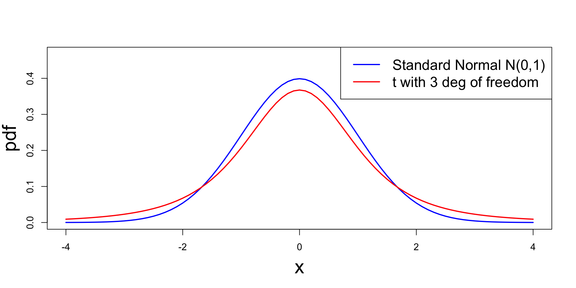
t-distribution

Comparison with Standard Normal

The t_p distribution approximates the standard normal N(0,1):

• t_p it is symmetric around zero and bell-shaped, like N(0,1)
• t_p has heavier tails compared to N(0,1)
• While the variance of N(0,1) is 1, the variance of t_p is \frac{p}{p-2}
• We have that t_p \to N(0,1) \quad \text{as} \quad p \to \infty

Plot: Comparison with Standard Normal

References

[1]

Casella, George, Berger, Roger L., Statistical inference, second edition, Brooks/Cole, 2002.

[2]

Gosset (Student), W.S., The probable error of a mean, Biometrika. 6 (1908) 1–25.