Statistical Models

Lecture 9

Dr. Silvio Fanzon

S.Fanzon@hull.ac.uk

University of Hull

Dr. John Fry

J.M.Fry@hull.ac.uk

University of Hull

Lecture 9:
General linear
regression

Outline of Lecture 9

1. General linear regression
2. Simple regression as general regression
3. Multiple linear regression
4. Coefficient of determination
5. Example of multiple regression
6. Two sample t-test as general regression

Part 1:
General linear
regression

Simple vs General regression

Simple regression:

• Response variable Y depends on one predictor X

• The goal is to learn distribution of

  Y | X

• Y | X allows to predict values of Y knowing values of X

Simple vs General regression

General regression:

• Response variable Y depends on p predictors

Z_1 , \ldots, Z_p

• The goal is to learn distribution of Y | Z_1, \ldots, Z_p

• Y | Z_1 , \dots, Z_p allows to predict Y knowing values of Z_1 , \dots, Z_p

General regression function

Suppose given random variables Z_1 , \ldots, Z_p and Y

• Z_1,\ldots, Z_p are the predictors

• Y is the response

Notation: We denote points of \mathbb{R}^p by z = (z_1, \ldots, z_p)

Definition

The regression function of Y on Z_1,\ldots,Z_p is the conditional expectation

R \colon \mathbb{R}^p \to \mathbb{R}\,, \qquad \quad R(z) := {\rm I\kern-.3em E}[Y | Z_1 = z_1, \ldots , Z_p = z_p]

General regression function

Idea

The regression function R(z) = {\rm I\kern-.3em E}[Y | Z_1 = z_1, \ldots , Z_p = z_p] predicts the most likely value of Y when we observe Z_1 = z_1, \ldots , Z_p = z_p

Notation: We use the shorthand {\rm I\kern-.3em E}[Y | z_1, \ldots, z_p] := {\rm I\kern-.3em E}[Y | Z_1 = z_1, \ldots , Z_p = z_p]

The general regression problem

Assumption: For each i =1 , \ldots, n we observe

• data point (z_{i1}, \ldots, z_{ip}, y_i)

• z_{ij} is from Z_j

• y_i is from Y

Problem

From the above data learn a regression function R(z) = {\rm I\kern-.3em E}[Y | z_1, \ldots, z_p] which explains the observations, that is, {\rm I\kern-.3em E}[Y | z_{i1}, \ldots, z_{ip}] \ \approx \ y_i \,, \qquad \forall \, i = 1 , \ldots, n

General linear regression

Key assumption: The regression function R(z) = {\rm I\kern-.3em E}[Y | z_1, \ldots, z_p] is linear

Definition

The regression of Y on Z_1 , \ldots, Z_p is linear if there exist \beta_1, \ldots, \beta_p s.t.

{\rm I\kern-.3em E}[Y | z_1, \ldots, z_p] = \beta_1 z_1 + \ldots + \beta_p z_p \,, \quad \forall \, z \in \mathbb{R}^p

\beta_1, \ldots, \beta_p are called regression coefficients

Note:

• In simple regression we have 2 coefficients \alpha and \beta

• In multiple regression we have p coefficients \beta_1, \ldots, \beta_p

General linear regression

Model Assumptions

Suppose that for each i =1 , \ldots, n we observe

• data point (z_{i1}, \ldots, z_{ip}, y_i)

• z_{ij} is from Z_j

• y_i is from Y

Definition

For each i = 1, \ldots, n we denote by Y_i a random variable with distribution Y | Z_1 = z_{i1} , \ldots, Z_p = z_{ip}

General linear regression

Model Assumptions

Assumptions:

1. Predictor is known: The values z_{i1}, \ldots, z_{ip} are known

2. Normality: The distribution of Y_i is normal

3. Linear mean: There are parameters \beta_1,\ldots,\beta_p such that {\rm I\kern-.3em E}[Y_i] = \beta_1 z_{i1} + \ldots + \beta_p z_{ip}

General linear regression

Model Assumptions

4. Common variance (Homoscedasticity): There is a parameter \sigma^2 such that {\rm Var}[Y_i] = \sigma^2

5. Independence: The random variables Y_1 \,, \ldots \,, Y_n are independent

Characterization of the Model

• Assumptions 1–5 look quite abstract
• The following Proposition gives a handy characterization

Proposition

Assumptions 1-5 are satisfied if and only if Y_i = \beta_1 z_{i1} + \ldots + \beta_p z_{ip} + \varepsilon_{i} for some errors \varepsilon_1 , \ldots, \varepsilon_n \,\, \text{ iid } \,\, N(0,\sigma^2)

Proof: Similar to the proof of Proposition in Slide 63 Lecture 8. Exercise

Likelihood function

Introduce the column vectors \beta := (\beta_1, \ldots, \beta_p)^T \,, \qquad y := (y_1,\ldots,y_n)^T

Proposition

Suppose Assumptions 1–5 hold. The likelihood of general linear regression is L(\beta, \sigma^2 | y ) = \frac{1}{(2\pi \sigma^2)^{n/2}} \, \exp \left( -\frac{\sum_{i=1}^n(y_i- \beta_1 z_{i1} - \ldots - \beta_p z_{ip})^2}{2\sigma^2} \right)

Likelihood function

Proof

• By assumption we have

Y_i \sim N(\beta_1 z_{i1} + \ldots + \beta_p z_{ip} , \sigma^2 )

• Therefore the pdf of Y_i is

f_{Y_i} (y_i) = \frac{1}{\sqrt{2\pi \sigma^2}} \exp \left( -\frac{(y_i - \beta_1 z_{i1} - \ldots - \beta_p z_{ip})^2}{2\sigma^2} \right)

Likelihood function

Proof

• Since Y_1,\ldots, Y_n are independent we obtain \begin{align*} L(\beta, \sigma^2 | y) & = f(y_1,\ldots,y_n) \\ & = \prod_{i=1}^n f_{Y_i}(y_i) \\ & = \prod_{i=1}^n \frac{1}{\sqrt{2\pi \sigma^2}} \exp \left( -\frac{(y_i - \beta_1 z_{i1} - \ldots - \beta_p z_{ip})^2}{2\sigma^2} \right) \\ & = \frac{1}{(2\pi \sigma^2)^{n/2}} \, \exp \left( -\frac{\sum_{i=1}^n(y_i- \beta_1 z_{i1} - \ldots - \beta_p z_{ip})^2}{2\sigma^2} \right) \end{align*}

• This concludes the proof

Design matrix

For each i = 1 , \ldots, n suppose given p observations z_{i1}, \ldots, z_{ip}

Definition

The design matrix is the n \times p matrix Z := \left( \begin{array}{ccc} z_{11} & \ldots & z_{1p} \\ z_{21} & \ldots & z_{2p} \\ \ldots & \ldots & \ldots \\ z_{n1} & \ldots & z_{np} \\ \end{array} \right)

Likelihood function

Vectorial notation

\begin{align*} y - Z\beta & = \left( \begin{array}{c} y_1 \\ y_2 \\ \ldots \\ y_n \\ \end{array} \right) - \left( \begin{array}{ccc} z_{11} & \ldots & z_{1p} \\ z_{21} & \ldots & z_{2p} \\ \ldots & \ldots & \ldots \\ z_{n1} & \ldots & z_{np} \\ \end{array} \right) \left( \begin{array}{c} \beta_1 \\ \ldots \\ \beta_p \\ \end{array} \right) \\[20pt] & = \left( \begin{array}{c} y_1 \\ y_2 \\ \ldots \\ y_n \\ \end{array} \right) - \left( \begin{array}{c} \beta_1 z_{11} + \ldots + \beta_p z_{1p}\\ \beta_1 z_{21} + \ldots + \beta_p z_{2p} \\ \ldots \\ \beta_1 z_{n1} + \ldots + \beta_p z_{np} \\ \end{array} \right) \\[20pt] & = \left( \begin{array}{c} y_1 - \beta_1 z_{11} - \ldots - \beta_p z_{1p}\\ y_2 - \beta_1 z_{21} - \ldots - \beta_p z_{2p} \\ \ldots \\ y_n - \beta_1 z_{n1} - \ldots - \beta_p z_{np} \\ \end{array} \right) \, \in \, \mathbb{R}^n \end{align*}

Likelihood function

Vectorial notation

From the previous calculation we get

(y - Z \beta)^T \, (y - Z\beta) = \sum_{i=1}^n \left( y_i - \beta_1 z_{i1} - \ldots - \beta_p z_{ip} \right)^2

Definition

Let Z be n \times p design matrix and y \in \mathbb{R}^n. The residual sum of squares associated to the parameter \beta is \mathop{\mathrm{RSS}}\colon \mathbb{R}^p \to \mathbb{R}\,, \qquad \mathop{\mathrm{RSS}}(\beta) := (y - Z \beta)^T \, (y - Z\beta)

Likelihood function

Vectorial notation

Using vectorial notation the likelihood function can be re-written as

\begin{align*} L(\beta, \sigma^2 | y ) & = \frac{1}{(2\pi \sigma^2)^{n/2}} \, \exp \left( -\frac{\sum_{i=1}^n(y_i - \beta_1 z_{i1} - \ldots - \beta_p z_{ip})^2}{2\sigma^2} \right) \\[20pt] & = \frac{1}{(2\pi \sigma^2)^{n/2}} \, \exp \left( - \frac{ (y - Z \beta)^T \, (y - Z\beta) }{2 \sigma^2} \right) \\[20pt] & = \frac{1}{(2\pi \sigma^2)^{n/2}} \, \exp \left( - \frac{\mathop{\mathrm{RSS}}(\beta) }{2 \sigma^2} \right) \end{align*}

General linear regression

Summary

• General linear regression of Y on Z_1, \ldots, Z_p is the function {\rm I\kern-.3em E}[Y | z_1,\ldots,z_p] = \beta_1 z_{1} + \ldots + \beta_p z_p

• For each i=1, \ldots, n suppose given the observations (z_{i1}, \ldots, z_{ip}, y_i)

General linear regression

Summary

• Denote by Y_i the random variable

Y | z_{i1} ,\ldots, z_{ip}

• Suppose that Y_i has the form

Y_i = \beta_1 z_{i1} + \ldots + \beta_p z_{ip} + \varepsilon_i

• The errors are

\varepsilon_1,\ldots, \varepsilon_n \,\, \text{ iid } \,\, N(0,\sigma^2)

The general linear regression problem

For each i = 1 , \ldots, n suppose given data points (z_{i1}, \ldots, z_{ip}, y_i)

Problem

From the above data learn a general linear regression function {\rm I\kern-.3em E}[Y | z_1, \ldots, z_p] = \beta_1 z_1 + \ldots + \beta_p z_p which explains the observations, that is, \begin{equation} \tag{5} {\rm I\kern-.3em E}[Y | z_{i1}, \ldots, z_{ip}] \ \approx \ y_i \,, \qquad \forall \, i = 1 , \ldots, n \end{equation}

Question

How do we enforce (5)?

Answer

• Recall that Y_i is distributed like

Y_i | z_{i1}, \ldots, z_{ip}

• Therefore

{\rm I\kern-.3em E}[Y | z_{i1}, \ldots, z_{ip}] = {\rm I\kern-.3em E}[Y_i]

• Hence (5) holds iff

\begin{equation} \tag{6} {\rm I\kern-.3em E}[Y_i] \ \approx \ y_i \,, \qquad \forall \, i = 1 , \ldots, n \end{equation}

Answer

• If we want (6) to hold, we need to maximize the joint probability

P(Y_1 \approx y_1, \ldots, Y_n \approx y_n)

• Recall that the likelihood for fixed y \in \mathbb{R}^n is defined as L(\beta, \sigma^2 | y) = f(y_1,\ldots,y_n)

• Thus joint probability is maximized iff likelihood is maximized

• Hence we need to find parameters \hat \beta, \hat \sigma which maximize the likelihood function

\max_{\beta,\sigma} \ L(\beta, \sigma^2 | y )

Maximizing the likelihood

Theorem

Suppose Assumptions 1–5 hold and assume given observations (z_{i1}, \ldots, z_{ip} ,y_i) \,, \qquad \quad \forall \, i =1 ,\ldots n \,, \qquad \det (Z Z^T) \neq 0 The maximization problem \max_{\beta,\sigma} \ L(\beta, \sigma^2 | y ) admits the unique solution \hat \beta = (Z^T Z)^{-1} Z^T y \,, \qquad \hat{\sigma}^2 = \frac{1}{n} \mathop{\mathrm{RSS}}(\hat \beta)

Minimizing the RSS

The proof of previous Theorem relies on the following Lemma

Lemma

Assume given observations (z_{i1}, \ldots, z_{ip} ,y_i) \,, \qquad \quad \forall \, i =1 ,\ldots n \,, \qquad \det (Z Z^T) \neq 0 The minimization problem \min_{\beta} \ \mathop{\mathrm{RSS}}(\beta) admits the unique solution \hat \beta = (Z^T Z)^{-1} Z^T y

Results from matrix calculus

• To prove the Lemma we need some auxiliary results

• In the following x denotes an n \times 1 column vector

x = \left( \begin{array}{c} x_1 \\ x_2 \\ \vdots \\ x_n \end{array} \right)

Results from matrix calculus

First result

• Suppose given an n \times 1 column vector a

• Define the scalar function

f \colon \mathbb{R}^n \to \mathbb{R}\,, \qquad f(x) := a^T x

• Then f is differentiable and the gradient is constant

\nabla f (x) = a^T

Results from matrix calculus

Second result

• Suppose given an m \times n matrix A

• Define the vectorial affine function

g \colon \mathbb{R}^n \to \mathbb{R}^m \,, \qquad g(x) := A x

• Then g is differentiable and the Jacobian is constant

J g (x) = A

Results from matrix calculus

Third result

• Suppose given an n \times n matrix M

• Define the quadratic form

h \colon \mathbb{R}^n \to \mathbb{R}\,, \qquad h(x) := x^T M x

• Then h is differentiable and the Jacobian is

J h(x) = x^T (M + M^T)

Additional results on the matrix transpose

1. For any m \times n matrix A (A^T)^T= A

2. Let M be a square n \times n matrix. Then M is symmetric iff M^T = M

3. Scalars can be seen as 1 \times 1 symmetric matrices

4. Therefore for any scalar c \in \mathbb{R} c^T = c

Additional results on the matrix transpose

5. For any m \times n matrix A and n \times p matrix B (AB)^T=B^T A^T

6. The matrix A^T A is symmetric by point (2) (A^T A)^T = A^T (A^T)^T = A^T A

Optimality conditions

We also need the n-dimensional version of the Lemma in Slide 18 Lecture 8

Lemma

Suppose f \colon \mathbb{R}^n \to \mathbb{R} has positive semi-definite Hessian. They are equivalent

1. The point \hat x is a minimizer of f, that is,

f( \hat x ) = \min_{x \in \mathbb{R}^n} f(x)

2. The point \hat x satisfies the optimality conditions

\nabla f (\hat x) = 0

Minimizing the RSS

Proof of Lemma

• We are finally ready to minimize the \mathop{\mathrm{RSS}}

\min_{\beta} \ \mathop{\mathrm{RSS}}(\beta)

• Recall that \mathop{\mathrm{RSS}}\colon \mathbb{R}^{p} \to \mathbb{R} with

\mathop{\mathrm{RSS}}(\beta) = (y - Z \beta)^T (y - Z \beta)

• It is not too difficult to show that \nabla^2 \mathop{\mathrm{RSS}} is positive-semidefinite

• The proof of this fact is left as an exercise

Minimizing the RSS

Proof of Lemma

• By the Lemma on Optimality Conditions in Slide 33

\beta \,\, \text{ minimizes } \,\, \mathop{\mathrm{RSS}}\qquad \iff \qquad \nabla \mathop{\mathrm{RSS}}(\beta) = 0

• To compute \nabla \mathop{\mathrm{RSS}} we first expand \mathop{\mathrm{RSS}}

\begin{align*} \mathop{\mathrm{RSS}}(\beta) & = (y-Z \beta)^T (y-Z \beta) \\[5pt] & = (y^T - (Z\beta)^T ) (y-Z \beta) \\[5pt] & = (y^T - \beta^T Z^T ) (y-Z \beta) \\[5pt] & = y^T y - y^T Z \beta - \beta^T Z^T y + \beta^T Z^T Z \beta \end{align*}

Minimizing the RSS

Proof of Lemma

• Note that
  • y has size n \times 1
  • Z has size n \times p
  • Therefore Z^T has size p \times n
  • \beta has size p \times 1
  • Thus \beta^T has size 1 \times p
• \beta^T Z^T y therefore has size

\left( 1 \times p \right) \times \left( p \times n \right) \times \left( n \times 1 \right) = 1 \times 1

Minimizing the RSS

Proof of Lemma

• \beta^T Z^T y \, is a scalar \quad \implies \quad it is symmetric and we get

\left( \beta^T Z^T y \right)^T = \beta^T Z^T y

• Using the properties of transposition we also get

\left( \beta^T Z^T y \right)^T = y^T Z \beta

• From the last 2 equations we conclude

y^T Z \beta = \beta^T Z^T y

Minimizing the RSS

Proof of Lemma

• The \mathop{\mathrm{RSS}} can now be written as

\begin{align*} \mathop{\mathrm{RSS}}(\beta) & = y^T y - y^T Z \beta - \textcolor{magenta}{\beta^T Z^T y} + \beta^T Z^T Z \beta \\[5pt] & = y^T y - y^T Z \beta - \textcolor{magenta}{y^T Z \beta} + \beta^T Z^T Z \beta \\[5pt] & = y^T y - 2 y^T Z \beta + \beta^T Z^T Z \beta \end{align*}

Minimizing the RSS

Proof of Lemma

• Therefore we have

\begin{align*} \nabla \mathop{\mathrm{RSS}}(\beta) & = \nabla ( y^T y ) - 2 \nabla (y^T Z \beta ) + \nabla (\beta^T Z^T Z \beta ) \\[5pt] & = - 2 \nabla (y^T Z \beta ) + \nabla (\beta^T Z^T Z \beta ) \end{align*}

• We need to compute

\nabla (y^T Z \beta ) \qquad \quad \text{ and } \qquad \quad \nabla (\beta^T Z^T Z \beta )

Minimizing the RSS

Proof of Lemma

• Note that y^T Z has dimension

( 1 \times n ) \times ( n \times p ) = 1 \times p

• Since \beta has dimension p \times 1 we can define the function

f \colon \mathbb{R}^p \to \mathbb{R}\,, \qquad f(\beta) := y^T Z \beta

• By the First Result on Matrix Calculus in Slide 28

\nabla f = \nabla ( \textcolor{magenta}{y^T Z} \beta) = \textcolor{magenta}{y^T Z}

Minimizing the RSS

Proof of Lemma

• Note that Z^T Z has dimension ( p \times n ) \times ( n \times p ) = p \times p

• Since \beta has dimension p \times 1 we can define the function

g \colon \mathbb{R}^p \to \mathbb{R}\,, \qquad g(\beta) := \beta^T Z^T Z \beta

• By the Third Result on Matrix Calculus in Slide 30

\begin{align*} \nabla h & = \nabla (\beta^T \textcolor{magenta}{Z^T Z} \beta) = \beta^T (\textcolor{magenta}{Z^T Z} + (\textcolor{magenta}{Z^T Z})^T ) \\[5pt] & = \beta^T ( Z^T Z + Z^T Z ) = 2 \beta^T (Z^T Z) \end{align*}

Minimizing the RSS

Proof of Lemma

• Putting together these results we obtain

\begin{align*} \nabla \mathop{\mathrm{RSS}}(\beta) & = - 2 \nabla (y^T Z \beta ) + \nabla (\beta^T Z^T Z \beta ) \\[5pt] & = -2 y^T Z + 2 \beta^T (Z^T Z) \end{align*}

• We can finally solve the optimality conditions:

\begin{align*} \nabla \mathop{\mathrm{RSS}}(\beta) = 0 \qquad & \iff \qquad -2 y^T Z + 2 \beta^T (Z^T Z) = 0 \\[5pt] & \iff \qquad \beta^T (Z^T Z) = y^T Z \end{align*}

Minimizing the RSS

Proof of Lemma

• So far we have

\beta^T (Z^T Z) = y^T Z

• Transposing both sides of the above equation yields

(Z^T Z) \beta = Z^T y

Minimizing the RSS

Proof of Lemma

• The matrix Z^T Z is invertible, since we are assuming

\det (Z^T Z) \neq 0

• Multiply by (Z^T Z)^{-1} both sides of

(Z^T Z) \beta = Z^T y

• We obtain

\beta = (Z^T Z)^{-1} Z^T y

Minimizing the RSS

Proof of Lemma

• In conclusion

\nabla \mathop{\mathrm{RSS}}(\beta) = 0 \qquad \iff \qquad \beta = (Z^T Z)^{-1} Z^T y

• By the Lemma on Optimality Conditions in Slide 33 we infer

\beta = (Z^T Z)^{-1} Z^T y \,\, \text{ minimizes } \,\, \mathop{\mathrm{RSS}}

• This concludes the proof

Maximizing the likelihood

We are finally in position to prove the main Theorem. We recall the statement

Theorem

Suppose Assumptions 1–5 hold and assume given observations such that (z_{i1}, \ldots, z_{ip} ,y_i) \,, \qquad \quad \forall \, i =1 ,\ldots n \,, \qquad \det (Z Z^T) \neq 0 The maximization problem \max_{\beta,\sigma} \ L(\beta, \sigma^2 | y ) admits the unique solution \hat \beta = (Z^T Z)^{-1} Z^T y \,, \qquad \hat{\sigma}^2 = \frac{1}{n} \mathop{\mathrm{RSS}}(\hat \beta)

Maximizing the likelihood

Proof of Theorem

• The \log function is strictly increasing

• Therefore the problem \max_{\beta,\sigma} \ L(\beta, \sigma^2 | y ) is equivalent to \max_{\beta,\sigma} \ \log L( \beta, \sigma^2 | y )

Maximizing the likelihood

Proof of Theorem

• Recall that the likelihood is

L(\beta, \sigma^2 | y ) = \frac{1}{(2\pi \sigma^2)^{n/2}} \, \exp \left( - \frac{ \mathop{\mathrm{RSS}}(\beta) }{2\sigma^2} \right)

• Hence the log–likelihood is

\log L(\beta, \sigma^2 | y ) = - \frac{n}{2} \log (2 \pi) - \frac{n}{2} \log \sigma^2 - \frac{ \mathop{\mathrm{RSS}}(\beta) }{2 \sigma^2}

Maximizing the likelihood

Proof of Theorem

Suppose \sigma is fixed. In this case the problem \max_{\beta} \ \left\{ \frac{n}{2} \log (2 \pi) - \frac{n}{2} \log \sigma^2 - \frac{ \mathop{\mathrm{RSS}}(\beta) }{2 \sigma^2} \right\} is equivalent to \min_{\beta} \ \mathop{\mathrm{RSS}}(\beta)

We have already seen that the \mathop{\mathrm{RSS}} is minimized at \hat \beta = (Z^T Z)^{-1} Z^T y

Maximizing the likelihood

Proof of Theorem

• Substituting \hat \beta we obtain

\begin{align*} \max_{\beta,\sigma} \ & \log L(\beta, \sigma^2 | y ) = \max_{\sigma} \ \log L(\hat \beta, \sigma^2 | y ) \\[5pt] & = \max_{\sigma} \ \left\{ - \frac{n}{2} \log (2 \pi) - \frac{n}{2} \log \sigma^2 - \frac{ \mathop{\mathrm{RSS}}(\hat \beta) }{2 \sigma^2} \right\} \end{align*}

• It can be shown that the unique solution to the above problem is \hat{\sigma}^2 = \frac{1}{n} \mathop{\mathrm{RSS}}(\hat \beta)

• This concludes the proof

Part 2:
Simple regression as
general regression

General linear regression model

• The general linear regression model is

Y_i = \beta_1 z_{i1} + \ldots + \beta_p z_{ip} + \varepsilon_i \,, \qquad i = 1 , \ldots, n

• Z is the design matrix of size n \times p

Z = \left( \begin{array}{ccc} z_{11} & \ldots & z_{1p} \\ \ldots & \ldots & \ldots \\ z_{n1} & \ldots & z_{np} \\ \end{array} \right)

General linear regression model

• The data column and parameters vectors are

y = \left( \begin{array}{c} y_1 \\ \ldots \\ y_{n} \\ \end{array} \right) \qquad \quad \beta = \left( \begin{array}{c} \beta_1 \\ \ldots \\ \beta_{p} \\ \end{array} \right)

• The likelihood for general linear regression is maximized by

\hat \beta = (Z^T Z)^{-1} Z^T y

Simple linear regression model

• The simple linear regression model is

Y_i = \alpha + \beta x_i + \varepsilon_i \,, \qquad i = 1 , \ldots, n

• The data is given by

x = \left( \begin{array}{c} x_1 \\ \ldots \\ x_{n} \\ \end{array} \right) \qquad \quad y = \left( \begin{array}{c} y_1 \\ \ldots \\ y_{n} \\ \end{array} \right)

• The likelihood for simple linear regression is maximized by

\hat \alpha = \overline{y} - \hat \beta \, \overline{x} \,, \qquad \quad \hat \beta = \frac{S_{xy}}{S_{xx}}

Simple linear regression from general

• The general regression model comprises the simple regression one

• To see this, consider a general linear model with p = 2 parameters

Y_i = \beta_1 z_{i1} + \beta_2 z_{i2} + \varepsilon_i \,, \qquad i = 1 , \ldots, n

• We want to compare the above to

Y_i = \alpha + \beta x_i + \varepsilon_i \,, \qquad i = 1 , \ldots, n

• The 2 models are equivalent iff

z_{i1} = 1 \,, \qquad z_{i2} = x_i \,, \qquad \forall \, i = 1 , \ldots, n

Simple linear regression from general

• Hence the design matrix is

Z = \left( \begin{array}{cc} 1 & x_{1} \\ \ldots & \ldots \\ 1 & x_{n} \\ \end{array} \right)

• Note that Z has size

n \times p = n \times 2

Simple linear regression from general

Goal

• Show that the multiple linear regression estimator (Z^T Z)^{-1} Z^T y recovers the simple linear regression estimators \hat \alpha = \overline{y} - \hat \beta \overline{x} \,, \qquad \quad \hat \beta = \frac{S_{xy}}{S_{xx}}

• We expect (Z^T Z)^{-1} Z^T y to contain the estimators \hat \alpha, \hat \beta

(Z^T Z)^{-1} Z^T y = \left( \begin{array}{cc} \hat \alpha \\ \hat \beta \end{array} \right)

Calculation of Z^T y

• Z has size n \times 2 \qquad \implies \qquad Z^T has size 2 \times n
• y has size n \times 1
• Therefore Z^T y has size

( 2 \times n ) \times (n \times 1) = 2 \times 1

Calculation of Z^T y

\begin{align*} Z^T y & = \left( \begin{array}{cc} 1 & x_1 \\ \ldots & \ldots\\ 1 & x_n \end{array} \right)^T \left( \begin{array}{l} y_1 \\ \ldots\\ y_n \end{array}\right) \\[15pt] & = \left( \begin{array}{ccc} 1 & \ldots & 1 \\ x_1 & \ldots & x_n \end{array} \right) \left( \begin{array}{l} y_1 \\ \ldots\\ y_n \end{array}\right) \\[15pt] & = \left(\begin{array}{c} 1 \times y_1 + 1 \times y_2 + \ldots + 1 \times y_n \\ x_1 y_1 + x_2 y_2 + \ldots + x_n y_n \end{array} \right) \\[15pt] & = \left( \begin{array}{c} n \overline{y} \\ \sum_{i=1}^n x_i y_i \end{array} \right) \end{align*}

Calculation of Z^T Z

• Z has size n \times 2
• Z^T has size 2 \times n
• Therefore Z^T Z has size

( 2 \times n ) \times (n \times 2) = 2 \times 2

Calculation of Z^T Z

\begin{align*} Z^T Z & = \left( \begin{array}{cc} 1 & x_1 \\ \ldots & \ldots\\ 1 & x_n \end{array} \right)^T \left( \begin{array}{cc} 1 & x_1 \\ \ldots & \ldots\\ 1 & x_n \end{array} \right) \\[15pt] & = \left( \begin{array}{ccc} 1 & \ldots & 1 \\ x_1 & \ldots & x_n \end{array} \right) \left( \begin{array}{cc} 1 & x_1 \\ \ldots & \ldots\\ 1 & x_n \end{array} \right) \\[15pt] & = \left( \begin{array}{cc} 1 \times 1 + \ldots + 1 \times 1 & 1 \times x_1 + \ldots + 1 \times x_n \\ x_1 \times 1 + \ldots + x_n \times 1 & x_1 \times x_1 + \ldots + x_n \times x_n \end{array} \right) \\[15pt] & = \left( \begin{array}{cc} n & n \overline{x} \\ n \overline{x} & \sum_{i=1}^n x_i^2 \end{array} \right) \end{align*}

Matrix inverse

• Suppose to have a 2 \times n matrix

M = \left( \begin{array}{cc} a & b \\ c & d \end{array} \right)

• M is invertible iff

\det M = ad - bc \neq 0

• If \det M \neq 0 the inverse of M is

M^{-1} = \frac{1}{ ad - bc} \left( \begin{array}{cc} d & -b \\ -c & a \end{array}\right)

Calculation of (Z^T Z)^{-1}

• The determinant of Z^T Z is

\begin{align*} \det \left( Z^T Z \right) & = \det \left( \begin{array}{cc} n & n \overline{x} \\ n \overline{x} & \sum_{i=1}^n x_i^2 \end{array} \right) \\[15pt] & = n \sum_{i=1}^n x^2_i - n^2 \overline{x}^2 \\[15pt] & = n S_{xx} \end{align*}

• Therefore we have

\det \left( Z^T Z \right) = n S_{xx} \geq 0

Calculation of (Z^T Z)^{-1}

• Notice that

S_{xx} = \sum_{i=1}^n (x_i - \overline{x})^2 = 0 \qquad \iff \qquad x_1 = \ldots = x_n = \overline{x}

• WLOG we can discard the trivial case S_{xx} = 0 because:
  • The predictors x_1, \ldots, x_n are either chosen or random
  • If they are chosen, it makes no sense to choose them all equal
  • If they are random, they will all be equal with probability 0

Calculation of (Z^T Z)^{-1}

• Therefore we assume S_{xx} > 0

• This way we have

\det \left( Z^T Z \right) = n S_{xx} > 0

• Thus Z^T Z is invertible with inverse

\begin{align*} (Z^T Z)^{-1} & = \left( \begin{array}{cc} n & n \overline{x} \\ n \overline{x} & \sum_{i=1}^n x_i^2 \end{array} \right)^{-1} \\[15pt] & = \frac{1}{n S_{xx} } \left( \begin{array}{cc} \sum_{i=1}^n x^2_i & -n \overline{x}\\ -n\overline{x} & n \end{array} \right) \end{align*}

Calculating (Z^T Z)^{-1} Z^T y

• (Z^T Z)^{-1} has size 2 \times 2

• Z^T y has size 2 \times 1

• (Z^T Z)^{-1} Z^T y therefore has dimensions (2 \times 2) \times (2 \times 1) = (2 \times 1)

• We expect (Z^T Z)^{-1} Z^T y to contain the simple regression estimators \hat \alpha, \hat \beta

(Z^T Z)^{-1} Z^T y = \left( \begin{array}{cc} \hat \alpha \\ \hat \beta \end{array} \right)

Calculating (Z^T Z)^{-1} Z^T y

• We have already computed (Z^T Z)^{-1} and Z^T y

• Their product is

(Z^T Z)^{-1} Z^T y = \frac{1}{n S_{xx} } \left( \begin{array}{cc} \sum_{i=1}^n x^2_i & -n \overline{x}\\ -n\overline{x} & n \end{array} \right) \left( \begin{array}{c} n \overline{y} \\ \sum_{i=1}^n x_i y_i \end{array} \right)

Calculating (Z^T Z)^{-1} Z^T y

• The first entry of (Z^T Z)^{-1} Z^T y is therefore

\begin{align*} \frac{ \sum_{i=1}^n x_i^2 n \overline{y} - n \overline{x} \sum_{i=1}^n x_i y_i }{n S_{xx}} & = \frac{ \sum_{i=1}^n x_i^2 \overline{y} - \overline{x} \sum_{i=1}^n x_i y_i }{ S_{xx}} \\[10pt] & = \frac{ \sum_{i=1}^n x_i^2 \overline{y} \textcolor{magenta}{- \overline{y} n \overline{x}^2 + \overline{y} n \overline{x}^2} - \overline{x} \sum_{i=1}^n x_i y_i }{ S_{xx}} \\[10pt] & = \overline{y} \ \frac{ \sum_{i=1}^n x_i^2 - n \overline{x}^2}{ S_{xx} } - \overline{x} \ \frac{ \sum_{i=1}^n x_i y_i - n \overline{x} \overline{y} }{ S_{xx} } \\[10pt] & = \overline{y} \ \frac{ S_{xx} }{ S_{xx} } - \overline{x} \ \frac{ S_{xy} }{ S_{xx} } \\[10pt] & = \overline{y} - \hat \beta \, \overline{x} = \hat{\alpha} \end{align*}

Calculating (Z^T Z)^{-1} Z^T y

• The second entry of (Z^T Z)^{-1} Z^T y is

\frac{ - n \overline{x} n \overline{y} + n \sum_{i=1}^n x_i y_i}{ n S_{xx} } = \frac{ \sum_{i=1}^n x_i y_i - n\overline{x} \overline{y} }{ S_{xx} } = \frac{ S_{xy} }{S_{xx}} = \hat{\beta}

• We have finally proven that

(Z^T Z)^{-1} Z^T y = \left( \begin{array}{cc} \hat \alpha \\ \hat \beta \end{array} \right)

• Conclusion
  • Simple linear regression can be seen as general regression with p = 2
  • Estimator for general regression recovers estimators for simple regression

Part 3:
Multiple linear
regression

Mutiple linear regression model

The response variable Y depends on p-1 predictors

X_2, \ldots, X_p

Note: We start counting from 2 for notational convenience

Assumption: For each i=1, \ldots, n we observe

• data point (x_{i2}, \ldots, x_{ip}, y_i)

• x_{ij} is from X_j

• y_i is from Y

Mutiple linear regression model

Denote by Y_i the random variable

Y | x_{i2} ,\ldots, x_{ip}

Definition

The multiple linear regression model is

Y_i = \beta_1 + \beta_2 x_{i2} + \ldots + \beta_p x_{ip} + \varepsilon_i

where the errors satisfy

\varepsilon_1,\ldots, \varepsilon_n \,\, \text{ iid } \,\, N(0,\sigma^2)

Mutiple vs General linear regression

• Multiple linear regression is a particular case of general linear regression

• To see this, consider a general linear model with p parameters

Y_i = \beta_1 z_{i1} + \beta_2 z_{i2} + \ldots + \beta_p z_{ip} + \varepsilon_i \,, \qquad i = 1 , \ldots, n

• We want to compare the above to

Y_i = \beta_1 + \beta_2 x_{i2} + \ldots + \beta_p x_{ip} + \varepsilon_i

• The 2 models are equivalent iff

z_{i1} = 1 \,, \qquad z_{i2} = x_{i2} \,, \qquad \ldots \qquad z_{ip} = x_{ip} \qquad \forall \, i = 1 , \ldots, n

Mutiple linear regression estimator

• Hence the design matrix Z and data vector y are

Z = \left( \begin{array}{cccc} 1 & x_{12} & \ldots & x_{1p} \\ 1 & x_{22} & \ldots & x_{2p} \\ \ldots & \ldots & \ldots & \ldots \\ 1 & x_{n2} & \ldots & x_{np} \\ \end{array} \right) \,, \qquad y = \left( \begin{array}{c} y_1 \\ \ldots \\ y_n \\ \end{array} \right)

• Note that
  • Z has size n \times p
  • y has size n \times 1
• The estimator for multiple regression is therefore \hat \beta \in \mathbb{R}^p

\hat \beta = (Z^T Z)^{-1} Z^T y

Part 4:
Coefficient of
determination

How good is the model?

• Consider the multiple linear regression model

Y_i = \beta_1 + \beta_2 x_{i2} + \ldots + \beta_p \, x_{ip} + \varepsilon_i

• Denote the estimator by

\hat \beta = (\hat \beta_1, \ldots, \hat \beta_p ) = (Z^T Z)^{-1} Z^T y

Problem

Quantify how well the model fits the observed values

y_1 , \ldots, y_n

Predicted values and RSS

• The predicted values are

\begin{align*} \hat y_i & := {\rm I\kern-.3em E}[ Y | x_{i2}, \ldots , z_{ip} ] \\ & = \hat \beta_1 + \hat \beta_2 \, x_{i2} + \ldots + \hat \beta_p \, x_{ip} \end{align*}

• Recall that the Residual sum of squares is

\mathop{\mathrm{RSS}}:= \sum_{i=1}^n ( y_i - \hat y_i )^2

• The \mathop{\mathrm{RSS}} measures deviation of predicted values from observed values

Explained sum of squares

• The explained sum of squares is

\mathop{\mathrm{ESS}}:= \sum_{i=1}^n ( \hat y_i - \overline{y} )^2

• \mathop{\mathrm{ESS}} measures deviation of predicted values from the grand mean

Total sum of squares

• The total sum of squares is

\mathop{\mathrm{TSS}}:= \sum_{i=1}^n ( y_i - \overline{y} )^2

• \mathop{\mathrm{TSS}} measures deviation of observed values from the grand mean

• Hence \mathop{\mathrm{TSS}} measures variability of the observed data y_1 , \ldots, y_n

\mathop{\mathrm{TSS}}= \mathop{\mathrm{ESS}}+ \mathop{\mathrm{RSS}}

Theorem

Suppose given the multiple regression linear model

Y_i = \beta_1 + \beta_2 x_{i2} + \ldots + \beta_p x_{ip} + \varepsilon_{i} for errors \varepsilon_1 , \ldots, \varepsilon_n iid N(0,\sigma^2). Then

\mathop{\mathrm{TSS}}= \mathop{\mathrm{ESS}}+ \mathop{\mathrm{RSS}}

Proof: Left as an exercise

Coefficient of determination

• The coefficient of determination is

R^2 := \frac{ \mathop{\mathrm{ESS}}}{ \mathop{\mathrm{TSS}}} = \frac{ \sum_{i=1}^n ( \hat y_i - \overline{y} )^2 }{ \sum_{i=1}^n ( y_i - \overline{y} )^2 }

• R^2 measures proportion of total data variability (\mathop{\mathrm{TSS}}) which is explained by the regression model (\mathop{\mathrm{ESS}})

• By the Theorem we have

R^2 = \frac{ \mathop{\mathrm{ESS}}}{ \mathop{\mathrm{TSS}}} = 1 - \frac{ \mathop{\mathrm{RSS}}}{ \mathop{\mathrm{TSS}}}

Coefficient of determination

Proposition

We have that

0 \leq R^2 \leq 1

Moreover

R^2 = 1 \qquad \iff \qquad y_i = \hat y_i \quad \,\, \forall \, i = 1 , \ldots, n

Coefficient of determination

Proof of Proposition

• Note that

\mathop{\mathrm{TSS}}, \, \mathop{\mathrm{ESS}}, \, \mathop{\mathrm{RSS}}\geq 0

• Therefore

R^2 := \frac{\mathop{\mathrm{ESS}}}{\mathop{\mathrm{TSS}}} \geq 0

Coefficient of determination

Proof of Proposition

• By the Theorem we also have

R^2 = \frac{ \mathop{\mathrm{ESS}}}{ \mathop{\mathrm{TSS}}} = 1 - \frac{ \mathop{\mathrm{RSS}}}{ \mathop{\mathrm{TSS}}} \leq 1

• Moreover note that

\mathop{\mathrm{RSS}}= \sum_{i=1}^n ( y_i - \hat y_i )^2 = 0 \qquad \iff \qquad y_i = \hat y_i \quad \,\, \forall \, i = 1 , \ldots, n

Coefficient of determination

Proof of Proposition

• The proof is concluded by noting that

\begin{align*} R^2 = 1 \quad & \iff \quad 1 - \frac{ \mathop{\mathrm{RSS}}}{ \mathop{\mathrm{TSS}}} = 1 \\[15pt] & \iff \quad \frac{ \mathop{\mathrm{RSS}}}{ \mathop{\mathrm{TSS}}} = 0 \\[15pt] & \iff \quad \mathop{\mathrm{RSS}}= 0 \\[15pt] & \iff \quad y_i = \hat y_i \quad \,\, \forall \, i = 1 , \ldots, n \end{align*}

Conclusion

We have shown that

• 0 \leq R^2 \leq 1

• R^2 = 1 \quad \iff \quad y_i = \hat y_i \quad \,\, \forall \, i = 1 , \ldots, n

Conclusion: R^2 measures how well the model fits the data

• R^2 close to 1 \quad \implies \quad model fits data well
• R^2 close to 0 \quad \implies \quad model does not fit data well

Part 5:
Example of
multiple regression

Example: Predicting unemployment

Goal: Predict unemployment rates

• Unemp. related to Productivity Index
• Other factors might also play a role
• These factors likely depend on the year
• Use year as surrogate for other factors

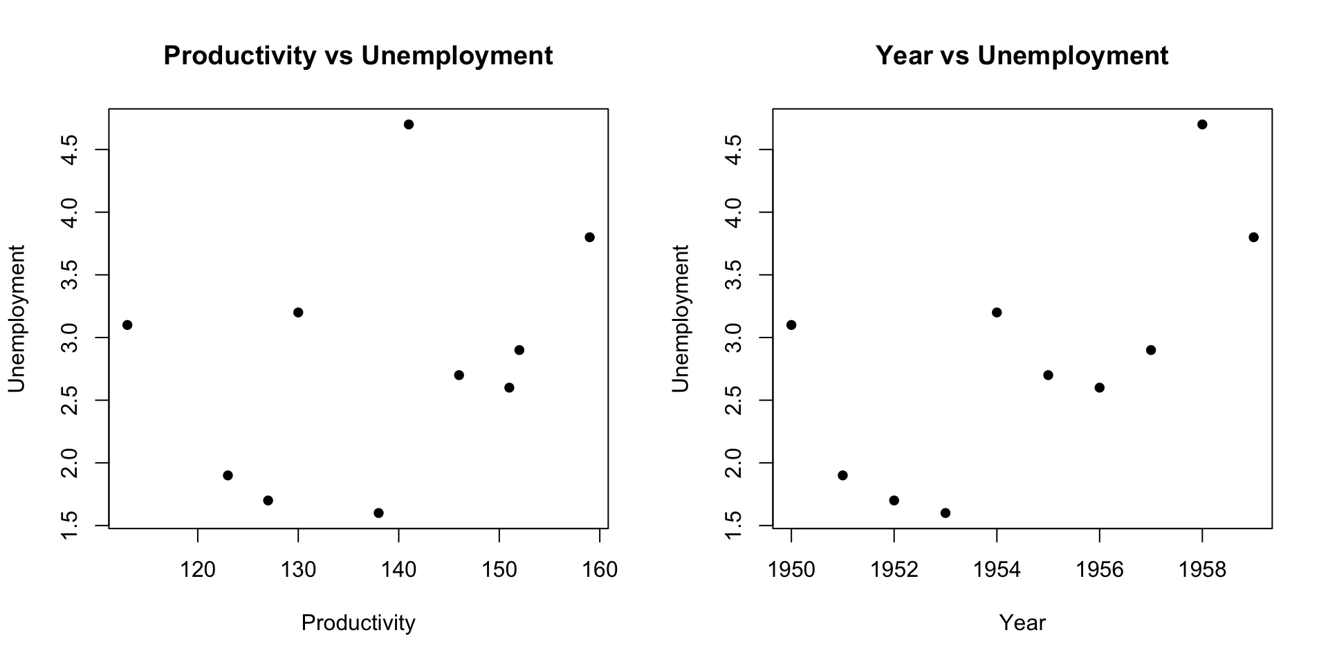
Unemp.	Product.	Year
3.1	113	1950
1.9	123	1951
1.7	127	1952
1.6	138	1953
3.2	130	1954
2.7	146	1955
2.6	151	1956
2.9	152	1957
4.7	141	1958
3.8	159	1959

Plotting the data

• Enter the data in 3 vectors

# Unemployment data
unemployment <- c(3.1, 1.9, 1.7, 1.6, 3.2, 2.7, 2.6, 2.9, 4.7, 3.8)

# Productivity data
productivity <- c(113, 123, 127, 138, 130, 146, 151, 152, 141, 159)

# Year data
year <- seq(1950, 1959, by = 1)

Plotting the data

• Using plot we plot productivity and year against unemployment

# Set up the layout with two plot panels side by side
par(mfrow = c(1, 2))

# Scatter plot: Productivity vs Unemployment
plot(productivity, unemployment, 
     xlab = "Productivity", ylab = "Unemployment",
     main = "Productivity vs Unemployment", 
     pch = 16)

# Scatter plot: Year vs Unemployment
plot(year, unemployment, 
     xlab = "Year", ylab = "Unemployment",
     main = "Year vs Unemployment", 
     pch = 16)

Plotting the data

There appears to be some relationship

Plotting the data in 3D

To better understand the data we can do a 3D scatter plot using either

• scatterplot3D
  • installed via install.packages("scatterplot3d")
  • produces static plots
• plotly
  • installed via install.packages("plotly")
  • produces interactive plots

Plotting the data with scatterplot3d

# Load the scatterplot3d library
library(scatterplot3d)

# Create 3D scatter plot
scatterplot3d(x = productivity,
              y = year,
              z = unemployment, 
              main = "Productivity and Year vs Unemployment", 
              xlab = "Productivity", 
              ylab = "Year", 
              zlab = "Unemployment",
              pch = 16,
              color = "black",
              angle = 50)

Plotting the data with scatterplot3d

Plotting the data with plotly

# Load the plotly library
library(plotly)

# Create a scatter plot using plot_ly
plot_ly(x = productivity, 
        y = year, 
        z = unemployment, 
        type = "scatter3d", 
        mode = "markers",
        marker = list(size = 5, color = "black")) %>%
  layout(scene = list(xaxis = list(title = "Productivity"),
                      yaxis = list(title = "Year"),
                      zaxis = list(title = "Unemployment")),
         width = 1000, 
         height = 500)

Plotting the data with plotly

The data is clearly close to a plane

Setting up multiple regression model

• We saw that the data points (x_i, y_i, z_i) = ( \text{productivity}, \text{year}, \text{unemployment} ) roughly lie on a plane

• Goal: Use multiple regression to model such plane

  • Unemployment is modelled by response variable Y
  • Productivity is modelled by predictor X_2
  • Year is modelled by predictor X_3
  • The multiple regression model is {\rm I\kern-.3em E}[Y | x_2, x_3] = \beta_1 + \beta_2 \, x_2 + \beta_3 \, x_3

Exercise

Multiple regression model is {\rm I\kern-.3em E}[Y | x_2, x_3] = \beta_1 + \beta_2 \, x_2 + \beta_3 \, x_3

• Enter design matrix Z into R
• Compute estimator \hat \beta = (Z^T Z)^{-1} Z^T y
• Matrix product in R is \,%*%
• Transpose matrix of \,A\, is \,t(A)
• Inverse of matrix \,A\, is \,solve(A)

Unemp.	Product.	Year
y_i	x_{i2}	x_{i3}
3.1	113	1950
1.9	123	1951
1.7	127	1952
1.6	138	1953
3.2	130	1954
2.7	146	1955
2.6	151	1956
2.9	152	1957
4.7	141	1958
3.8	159	1959

Solution

The design matrix is Z=\left(\begin{array}{cccc} 1 & 113 & 1950 \\ 1 & 123 & 1951 \\ 1 & 127 & 1952 \\ 1 & 138 & 1953 \\ 1 & 130 & 1954 \\ 1 & 146 & 1955 \\ 1 & 151 & 1956 \\ 1 & 152 & 1957 \\ 1 & 141 & 1958 \\ 1 & 159 & 1959 \\ \end{array}\right)

Unemp.	Product.	Year
y_i	x_{i2}	x_{i3}
3.1	113	1950
1.9	123	1951
1.7	127	1952
1.6	138	1953
3.2	130	1954
2.7	146	1955
2.6	151	1956
2.9	152	1957
4.7	141	1958
3.8	159	1959

Solution

The data vector is y = \left(\begin{array}{c} 3.1 \\ 1.9 \\ 1.7 \\ 1.6 \\ 3.2 \\ 2.7 \\ 2.6 \\ 2.9 \\ 4.7 \\ 3.8 \\ \end{array}\right)

Unemp.	Product.	Year
y_i	x_{i2}	x_{i3}
3.1	113	1950
1.9	123	1951
1.7	127	1952
1.6	138	1953
3.2	130	1954
2.7	146	1955
2.6	151	1956
2.9	152	1957
4.7	141	1958
3.8	159	1959

Solution

Data vector y is stored in R as usual

# Store vector y
y <- c(3.1, 1.9, 1.7, 1.6, 3.2, 2.7, 2.6, 2.9, 4.7, 3.8)

Solution

Design matrix is stored as follows

# Store design matrix Z as long vector
Z <- c(1, 113, 1950,
       1, 123, 1951,
       1, 127, 1952,
       1, 138, 1953,
       1, 130, 1954,
       1, 146, 1955,
       1, 151, 1956,
       1, 152, 1957,
       1, 141, 1958,
       1, 159, 1959)

# Make Z into a matrix with 3 columns
Z <- matrix(Z, ncol = 3, byrow = TRUE)

Solution

• We need to compute the estimator

\hat \beta = (Z^T Z)^{-1} Z^T y

• The matrix transpose is computed with \,t(A)
• The product of two matrices A and B is computed with \, A %*% B
• We use these two operators to compute Z^T Z and store it into m1

# Calculate m1
m1 <- t(Z) %*% Z

Solution

• The inverse of a matrix A is computed with \, solve(A)
• We use this function to compute (Z^T Z)^{-1} and store it into m2

# Calculate m2
m2 <- solve(m1)

• We can compute Z^T y with \,%*%
• This is because R automatically interprets vectors as matrices

# Calculate m3
m3 <- t(Z) %*% y

Solution

• We compute the estimator \hat{\beta}=(Z^T Z)^{-1} Z^T y and store it as \, beta

# Calculate estimator beta
beta <- m2 %*% m3

• We then print the result to screen

# Print estimator beta
cat("The estimator is", beta)

The estimator is -1271.75 -0.1033386 0.6594171

Solution

• The computed regression model is

\begin{align*} {\rm I\kern-.3em E}[Y | x_2, x_3] & = \hat\beta_1 + \hat\beta_2 \, x_2 + \hat\beta_3 \, x_3 \\[15pt] & = -1271.75 + -0.1033386 \times x_2 + 0.6594171 \times x_3 \end{align*}

• Previous code can be downloaded here multiple_regression.R

Solution: Plot of data and regression plane

# Load the plotly library
library(plotly)

# Data
unemployment <- c(3.1, 1.9, 1.7, 1.6, 3.2, 2.7, 2.6, 2.9, 4.7, 3.8)
productivity <- c(113, 123, 127, 138, 130, 146, 151, 152, 141, 159)
year <- seq(1950, 1959, by = 1)

# Generate a grid of x and y values
x_grid <- seq(min(productivity), max(productivity), length.out = 50)
y_grid <- seq(min(year), max(year), length.out = 50)
grid <- expand.grid(productivity = x_grid, year = y_grid)

# Calculate z values for the regression plane
z_values <- -1271.75 - 0.1033386 * grid$productivity + 0.6594171 * grid$year

# Create a scatter plot using plot_ly
plot_ly(x = productivity, 
        y = year, 
        z = unemployment, 
        type = "scatter3d", 
        mode = "markers",
        marker = list(size = 5, color = "black")) %>%
  layout(scene = list(xaxis = list(title = "Productivity"),
                      yaxis = list(title = "Year"),
                      zaxis = list(title = "Unemployment")),
         width = 1000, 
         height = 500) %>%
         add_surface(
         x = x_grid, 
         y = y_grid, 
         z = matrix(z_values, nrow = length(x_grid)),
         opacity = 0.5, 
         colorscale = list(c(0, 'rgb(255,255,255)'), c(1, 'rgb(255,0,0)')))

Computing the R^2 coefficient

• How well does such multiple linear model fit our data?

• To answer this question we compute the coefficient of determination

R^2 = \frac{ \mathop{\mathrm{ESS}}}{ \mathop{\mathrm{TSS}}} = \frac{ \sum_{i=1}^n ( \hat y_i - \overline{y} )^2 }{ \sum_{i=1}^n (y_i - \overline{y})^2 }

Computing \mathop{\mathrm{TSS}}

• We have that

\mathop{\mathrm{TSS}}:= \sum_{i=1}^n (y_i - \overline{y})^2

• We compute \overline{y} with the R command

# Compute mean of y
y_bar <- mean(y)

• We compute \mathop{\mathrm{TSS}} with the R command

# Compute TSS
TSS <- sum( ( y - y_bar) ^ 2 )

Computing \mathop{\mathrm{ESS}}

• We have that

\mathop{\mathrm{ESS}}:= \sum_{i=1}^n (\hat y_i - \overline{y})^2

• We need to compute

\hat y_i := \hat \beta_1 + \hat \beta_2 x_{i2} + \hat \beta_3 x_{i3}

Computing \mathop{\mathrm{ESS}}

• \hat y, the design matrix Z, and \hat \beta are

\hat y = \left(\begin{array}{c} \hat y_1 \\ \ldots \\ \hat y_i \\ \ldots \\ \hat y_n \\ \end{array}\right) \,, \qquad Z = \left(\begin{array}{cccc} 1 & x_{11} & x_{12} \\ \ldots & \ldots & \ldots \\ 1 & x_{i1} & x_{i2} \\ \ldots & \ldots & \ldots \\ 1 & x_{n1} & x_{n2} \\ \end{array}\right) \,, \qquad \hat \beta = \left(\begin{array}{c} \hat \beta_1 \\ \hat \beta_2 \\ \hat \beta_3 \\ \end{array}\right)

• Therefore we can compute \hat y_i = \hat \beta_1 + \hat \beta_2 x_{i2} + \hat \beta_3 x_{i3} with the product \hat y = Z \hat \beta

Computing \mathop{\mathrm{ESS}}

• Recall that \hat \beta is stored in beta

• Therefore we can compute \hat y with R command

# Compute predictions y hat
y_hat <- Z %*% beta

• Finally \mathop{\mathrm{ESS}} is computed with

# Compute ESS
ESS <- sum( (y_hat - y_bar) ^ 2 )

Computing R^2

• The coefficient R^2 is computed with

# Compute coefficient of determination R^2
R2 <- ESS / TSS

# Print ESS, RSS and R^2
cat("\nThe Estimated Squared Error ESS is", ESS)
cat("\nThe Total Squared Error TSS is", TSS)
cat("\nThe coefficient of determination R^2 is", R2)

• The full code can be downloaded here R2_multiple_regression.R

Computing R^2

• Running the code we obtain the output

The estimator is -1271.75 -0.1033386 0.6594171

The Estimated Squared Error ESS is 7.249764

The Total Squared Error TSS is 8.376

The coefficient of determination R^2 is 0.8655401

• In particular we have

R^2 = 0.8655401

Conclusions

The coefficient of determination

R^2 = 0.8655401

is quite close to 1, showing that

• The model fits data quite well
• Productivity Index and Year affect Unemployment
• Unemployment is almost completely explained by Productivity Index and Year

Part 6:
Two sample t-test
as general regression

Two-sample t-test as general regression

• Two-sample t-test is particular case of general linear regression

• This example is important for two reasons

  • Shows that multiple linear regression encapsulates simple models like the two-sample t-test
  • Shows that general linear regression leads to intuitive solutions in simple examples

Two-sample t-test setting

• We have 2 populations A and B distributed like N(\mu_A, \sigma_A^2) and N(\mu_B, \sigma_B^2)

• We have two samples

  • Sample of size n_A from population A a = (a_1, \ldots, a_{n_A})
  • Sample of size n_B from population B b = (b_1, \ldots, b_{n_B})

• Two-sample t-test compares means \mu_A and \mu_B by computing t-statistic t = \frac{ \overline{a} - \overline{b} }{\mathop{\mathrm{e.s.e.}}}

Setting up the regression analysis

• We want a regression model that can describe the sample means \overline{a} and \overline{b}

• To this end, we fit a general linear model with p = 2 to the data

{\rm I\kern-.3em E}[Y | Z_1 = z_1 , Z_2 = z_2 ] = \beta_1 z_1 + \beta_2 z_2

• Define the data vector y by concatenating a and b

y = \left(\begin{array}{c} y_1 \\ \ldots \\ y_{n_A} \\ y_{n_A + 1}\\ \ldots \\ y_{n_A + n_B} \end{array}\right) = \left(\begin{array}{c} a_1 \\ \ldots \\ a_{n_A} \\ b_{1}\\ \ldots \\ b_{n_B} \end{array}\right)

Setting up the regression analysis

• The variable Z_1 is modelled as

Z_1 = 1_{A}(i) := \begin{cases} 1 & \text{ if i-th observation is from population A} \\ 0 & \text{ otherwise} \end{cases}

• Therefore we have

\begin{align*} z_1 & = (\underbrace{1_A(i) , \ldots, 1_A(i)}_{n_A + n_B} ) \\[15pts] & = (\underbrace{1 , \ldots, 1}_{n_A}, \underbrace{0 , \ldots, 0}_{n_B} ) \end{align*}

Setting up the regression analysis

• Similarly, the variable Z_2 is modelled as

Z_2 = 1_{B}(i) := \begin{cases} 1 & \text{ if i-th observation is from population B} \\ 0 & \text{ otherwise} \end{cases}

• Therefore we have

\begin{align*} z_2 & = (\underbrace{1_B(i), \ldots, 1_B (i)}_{n_A + n_B} ) \\[15pts] & = (\underbrace{0 , \ldots, 0}_{n_A}, \underbrace{1 , \ldots, 1}_{n_B} ) \end{align*}

Setting up the regression analysis

• The general regression model is

Y_i = \beta_1 \, 1_{A}(i) + \beta_2 \, 1_{B}(i) + \varepsilon_i

• Variables 1_A and 1_B are called dummy variables (more on this later)

• The design matrix is therefore

Z = (1_A | 1_B) = \left(\begin{array}{cc} 1_A(i) & 1_B (i) \\ \ldots & \ldots\\ 1_A(i) & 1_B (i) \\ \end{array}\right) = \left(\begin{array}{cc} 1 & 0 \\ \ldots & \ldots\\ 1 & 0\\ 0 & 1 \\ \ldots & \ldots\\ 0 & 1 \end{array}\right)

Calculation of Z^T y

• We want to compute the regression estimator

\hat \beta = (Z^T Z)^{-1} Z^T y

• Z has dimension (n_A + n_B) \times 2
• Z^T has dimension 2 \times (n_A + n_B)
• y has dimension (n_A + n_B) \times 1
• Z^T y therefore has dimension

[ 2 \times (n_A + n_B)] \times [ (n_A + n_B) \times 1 ] = 2 \times 1

Calculation of Z^T y

\begin{align*} Z^T y & = \left(\begin{array}{cc} 1 & 0 \\ \ldots & \ldots\\ 1 & 0\\ 0 & 1\\ \ldots & \ldots\\ 0 & 1 \end{array}\right)^T \left(\begin{array}{c} y_1 \\ \ldots\\ y_{n_A}\\ y_{n_A+1}\\ \ldots\\ y_{n_A+n_B} \end{array}\right) = \left(\begin{array}{cccccc} 1 & \ldots & 1 & 0 & \ldots & 0 \\ 0 & \ldots & 0 & 1 & \ldots & 1 \\ \end{array}\right) \left(\begin{array}{c} y_1 \\ \ldots\\ y_{n_A}\\ y_{n_A+1}\\ \ldots\\ y_{n_A+n_B} \end{array}\right) \\[35pt] & = \left(\begin{array}{c} y_1 \cdot 1 + \ldots + y_{n_A} \cdot 1 + y_{n_A + 1} \cdot 0 + \ldots + y_{n_A + n_B} \cdot 0 \\ y_1 \cdot 0 + \ldots + y_{n_A} \cdot 0 + y_{n_A + 1} \cdot 1 + \ldots + y_{n_A + n_B} \cdot 1 \end{array}\right) \\[20pt] & = \left(\begin{array}{c} y_1 + \ldots + y_{n_A} \\ y_{n_A + 1} + \ldots + y_{n_A + n_B} \end{array}\right) = \left(\begin{array}{c} a_1 + \ldots + a_{n_A} \\ b_{1} + \ldots + b_{n_B} \end{array}\right) = \left(\begin{array}{c} n_A \ \overline{a} \\ n_B \ \overline{b} \end{array}\right) \end{align*}

Calculation of Z^T Z

• Z has dimension (n_A + n_B) \times 2
• Z^T has dimension 2 \times (n_A + n_B)
• Z^T Z therefore has dimension [ 2 \times (n_A + n_B)] \times [ (n_A + n_B) \times 2 ] = 2 \times 2

Calculation of Z^T Z

\begin{align*} Z^T Z & = \left(\begin{array}{cc} 1 & 0 \\ \ldots & \ldots\\ 1 & 0\\ 0 & 1\\ \ldots & \ldots\\ 0 & 1 \end{array}\right)^T \left(\begin{array}{cc} 1 & 0 \\ \ldots & \ldots\\ 1 & 0\\ 0 & 1\\ \ldots & \ldots\\ 0 & 1 \end{array}\right) \\[35pt] & = \left(\begin{array}{cccccc} 1 & \ldots & 1 & 0 & \ldots & 0 \\ 0 & \ldots & 0 & 1 & \ldots & 1 \\ \end{array}\right) \left(\begin{array}{cc} 1 & 0 \\ \ldots & \ldots\\ 1 & 0\\ 0 & 1\\ \ldots & \ldots\\ 0 & 1 \end{array}\right) = \left(\begin{array}{cc} n_A & 0 \\ 0 & n_B \end{array}\right) \end{align*}

Calculation of \hat \beta

• The inverse of a diagonal matrix is diagonal

(Z^T Z)^{-1} = \left(\begin{array}{cc} n_A & 0 \\ 0 & n_B \end{array}\right)^{-1} =\left(\begin{array}{cc} \frac{1}{n_A} & 0 \\ 0 & \frac{1}{n_B} \end{array}\right)

• Then we can calculate

\hat \beta = (Z^T Z)^{-1} Z^Ty = \left(\begin{array}{cc} \frac{1}{n_A} & 0 \\ 0 & \frac{1}{n_B} \end{array}\right) \left(\begin{array}{c} n_A \ \overline{a} \\ n_B \ \overline{b} \end{array}\right) = \left(\begin{array}{c} \overline{a} \\ \overline{b} \end{array}\right)

Conclusions

• Therefore the estimator is

\hat \beta = \left(\begin{array}{c} \overline{a} \\ \overline{b} \end{array}\right)

• The regression function is hence

\begin{align*} {\rm I\kern-.3em E}[Y | 1_A = z_1 , 1_B = z_2] & = \hat\beta_1 \ z_1 + \hat\beta_2 \ z_2 \\[20pt] & = \overline{a} \ z_1 + \overline{b} \ z_2 \end{align*}

Conclusions

• This is a very intuitive result:
  • The expected value for Y when data is observed from population A is {\rm I\kern-.3em E}[Y | 1_A = 1 , 1_B = 0] = \overline{a}
  • The expected value for Y when data is observed from population B is {\rm I\kern-.3em E}[Y | 1_A = 0 , 1_B = 1] = \overline{b}
• Therefore, under this simple model
  • The best estimate for population A is the sample mean \overline{a}
  • The best estimate for population B is the sample mean \overline{b}