Statistical Models
Lecture 8
Lecture 8:
The maths of
regression
Outline of Lecture 8
- Least squares
- Simple linear regression
Part 1:
Least squares
Example: Blood Pressure
10 patients are treated with Drug A and Drug B
- These drugs cause change in blood pressure
- Patients are given the drugs one at a time
- Changes in blood pressure are recorded
- For patient i we denote by
- x_i the change caused by Drug A
- y_i the change caused by Drug B
| i | x_i | y_i |
|---|---|---|
| 1 | 1.9 | 0.7 |
| 2 | 0.8 | -1.0 |
| 3 | 1.1 | -0.2 |
| 4 | 0.1 | -1.2 |
| 5 | -0.1 | -0.1 |
| 6 | 4.4 | 3.4 |
| 7 | 4.6 | 0.0 |
| 8 | 1.6 | 0.8 |
| 9 | 5.5 | 3.7 |
| 10 | 3.4 | 2.0 |
Example: Blood Pressure
Goal:
- Predict reaction to Drug B, knowing reaction to Drug A
- This means predict y_i from x_i
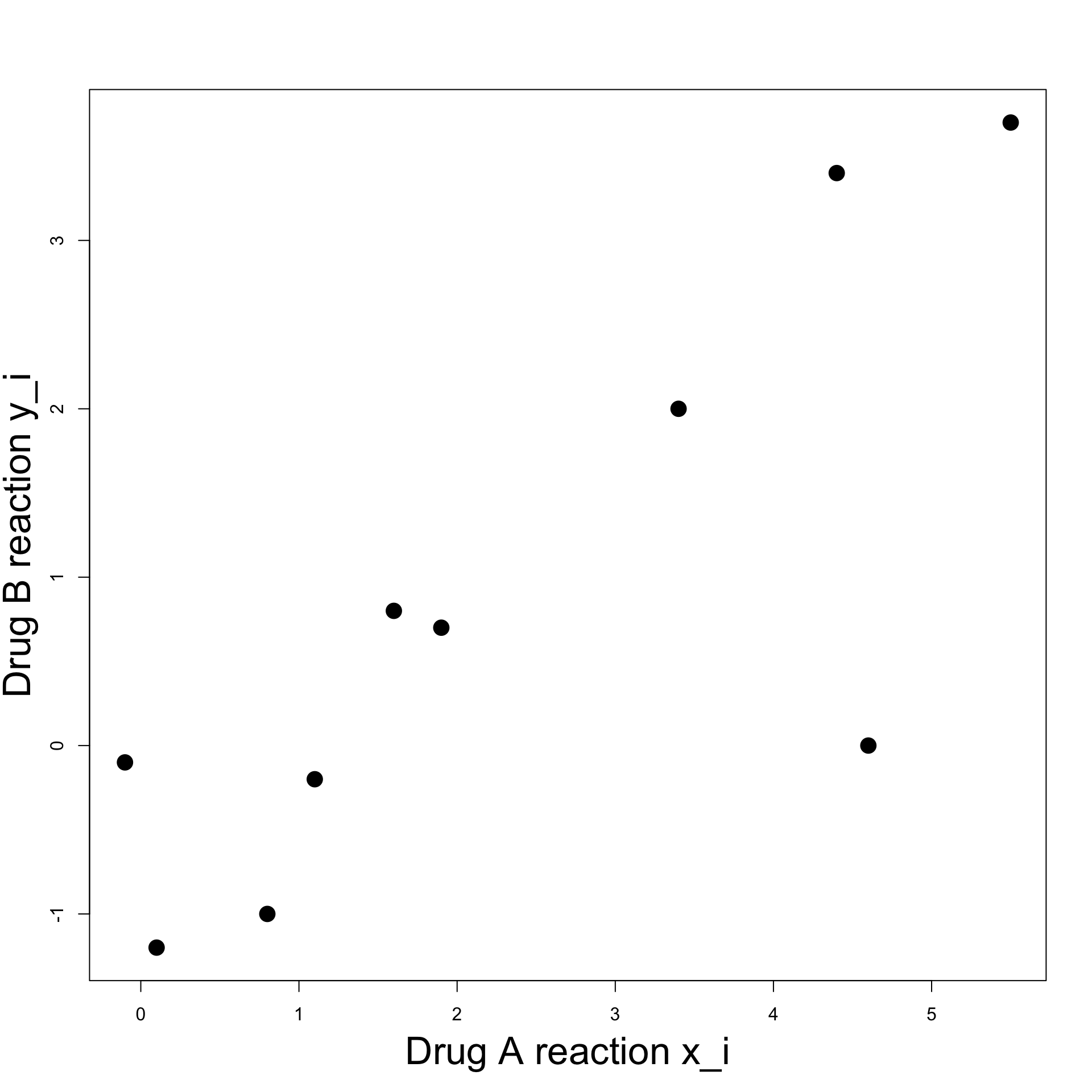
Plot:
- To visualize data we can plot pairs (x_i,y_i)
- Points seem to align
- It seems there is a linear relation between x_i and y_i
Example: Blood Pressure
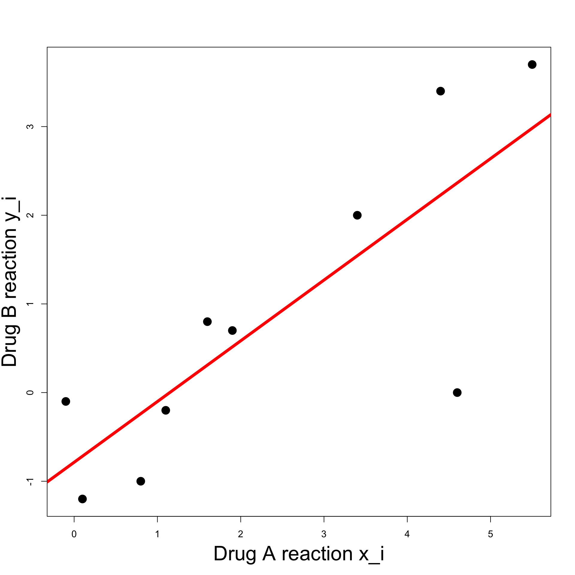
Linear relation:
- Try to fit a line through the data
- Line roughly predicts y_i from x_i
- However note the outlier (x_7,y_7) = (4.6, 0)
- How is such line constructed?
Example: Blood Pressure
Least Squares Line:
- A general line has equation
y = \beta x + \alpha
for some
- slope \beta
- intercept \alpha
- Value predicted by the line for x_i is \hat{y}_i = \beta x_i + \alpha
Example: Blood Pressure
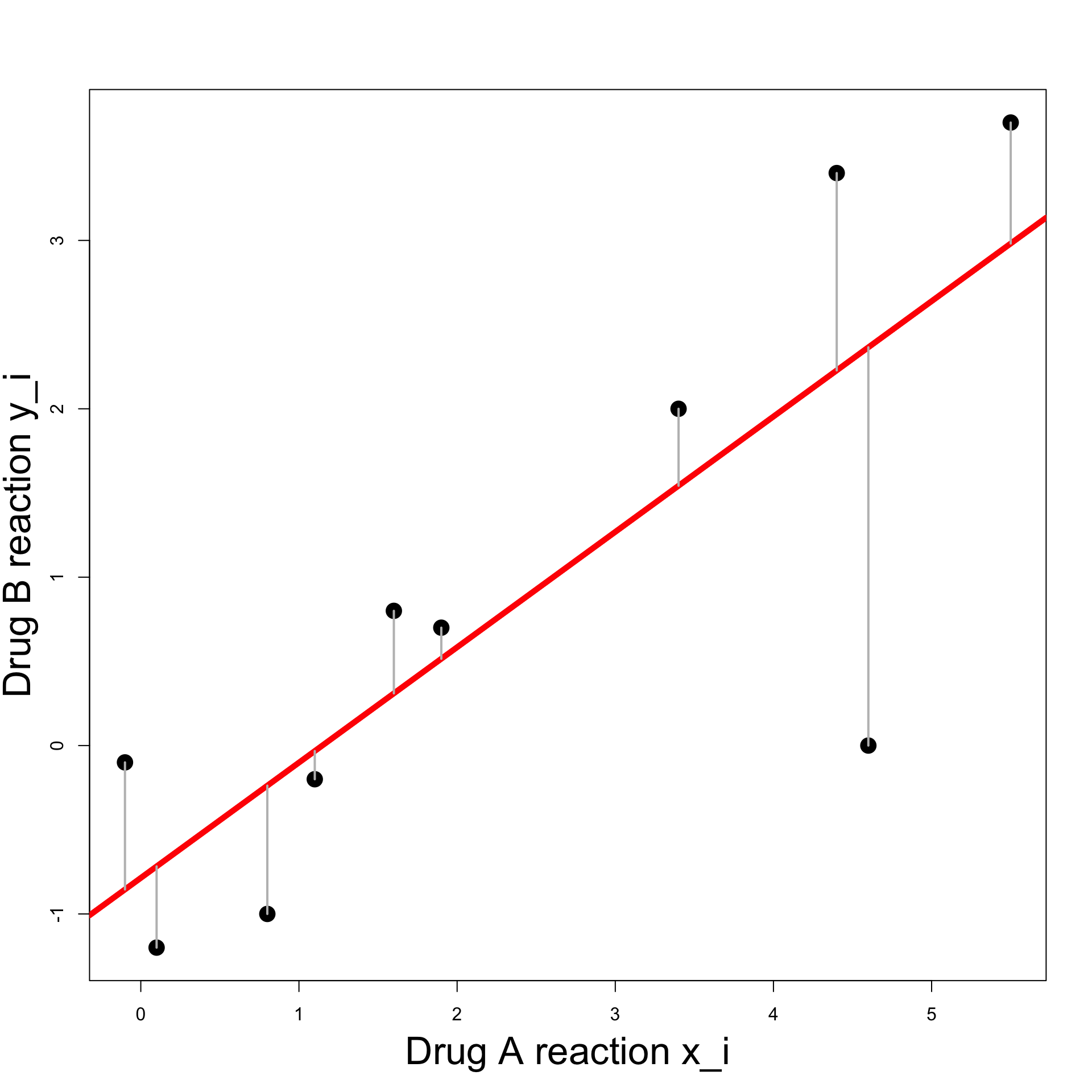
Least Squares Line:
We would like predicted and actual value to be close \hat{y}_i \approx y_i
Hence the vertical difference has to be small y_i - \hat{y}_i \approx 0

Example: Blood Pressure
Least Squares Line:
We want \hat{y}_i \approx y_i \,, \qquad \forall \, i
A way to ensure the above is by minimizing the sum of squares \min_{\alpha, \beta} \ \sum_{i} \ (y_i - \hat{y}_i)^2 \hat{y}_i = \beta x_i + \alpha

Residual Sum of Squares
Definition
Let (x_1,y_1), \ldots, (x_n, y_n) be a set of n points. Consider the line
y = \beta x + \alpha
The Residual Sum of Squares associated to the line is
\mathop{\mathrm{RSS}}(\alpha,\beta) := \sum_{i=1}^n (y_i-\alpha-{\beta}x_i)^2
Note: \mathop{\mathrm{RSS}} can be seen as a function \mathop{\mathrm{RSS}}\colon \mathbb{R}^2 \to \mathbb{R}\qquad \quad \mathop{\mathrm{RSS}}= \mathop{\mathrm{RSS}}(\alpha,\beta)
\mathop{\mathrm{RSS}}(\alpha,\beta) for Blood Pressure data
Summary statistics
Suppose given the sample (x_1,y_1), \ldots, (x_n, y_n)
We want to minimize the associated RSS \min_{\alpha,\beta} \ \mathop{\mathrm{RSS}}(\alpha,\beta) = \min_{\alpha,\beta} \ \sum_{i=1}^n (y_i-\alpha-{\beta}x_i)^2
To this end we define the following quantities
Summary statistics
Suppose given the sample (x_1,y_1), \ldots, (x_n, y_n)
Sample Means: \overline{x} := \frac{1}{n} \sum_{i=1}^n x_i \qquad \quad \overline{y} := \frac{1}{n} \sum_{i=1}^n y_i
Sums of squares: S_{xx} := \sum_{i=1}^n ( x_i - \overline{x} )^2 \qquad \quad S_{yy} := \sum_{i=1}^n ( y_i - \overline{y} )^2
Summary statistics
Suppose given the sample (x_1,y_1), \ldots, (x_n, y_n)
- Sum of cross-products: S_{xy} := \sum_{i=1}^n ( x_i - \overline{x} ) ( y_i - \overline{y} )
Minimizing the RSS
Theorem
Let (x_1,y_1), \ldots, (x_n, y_n) be a set of n points. Consider the minimization problem \begin{equation} \tag{M} \min_{\alpha,\beta } \ \mathop{\mathrm{RSS}}= \min_{\alpha,\beta} \ \sum_{i=1}^n (y_i-\alpha-{\beta}x_i)^2 \end{equation} Then
- There exists a unique line solving (M)
- Such line has the form y = \hat{\beta} x + \hat{\alpha} with \hat{\beta} = \frac{S_{xy}}{S_{xx}} \qquad \qquad \hat{\alpha} = \overline{y} - \hat{\beta} \ \overline{x}
Positive semi-definite matrix
To prove the Theorem we need some background results
A symmetric matrix is positive semi-definite if all the eigenvalues \lambda_i satisfy \lambda_i \geq 0
Proposition: A 2 \times 2 symmetric matrix M is positive semi-definite iff \det M \geq 0 \,, \qquad \quad \operatorname{Tr}(M) \geq 0
Positive semi-definite Hessian
- Suppose given a smooth function of 2 variables
f \colon \mathbb{R}^2 \to \mathbb{R}\qquad \quad f = f (x,y)
- The Hessian of f is the matrix
\nabla^2 f = \left( \begin{array}{cc} f_{xx} & f_{xy} \\ f_{yx} & f_{yy} \\ \end{array} \right)
Positive semi-definite Hessian
- In particular the Hessian is positive semi-definite iff
\det \nabla^2 f = f_{xx} f_{yy} - f_{xy}^2 \geq 0 \qquad \quad f_{xx} + f_{yy} \geq 0
- Side Note: For C^2 functions it holds that
\nabla^2 f \, \text{ is positive semi-definite} \qquad \iff \qquad f \, \text{ is convex}
Optimality conditions
Lemma
Suppose f \colon \mathbb{R}^2 \to \mathbb{R} has positive semi-definite Hessian. They are equivalent
The point (\hat{x},\hat{y}) is a minimizer of f, that is, f(\hat{x}, \hat{y}) = \min_{x,y} \ f(x,y)
The point (\hat{x},\hat{y}) satisfies the optimality conditions \nabla f (\hat{x},\hat{y}) = 0
Note: The proof of the above Lemma can be found in [1]
Optimality conditions
Example
- The main example of strictly convex function in 2D is
f(x,y) = x^2 + y^2
- It is clear that
\min_{x,y} \ f(x,y) = \min_{x,y} \ x^2 + y^2 = 0 with the only minimizer being (0,0)
- However let us use the Lemma to prove this fact
Optimality conditions
Example
- The gradient of f = x^2 + y^2 is
\nabla f = (f_x,f_y) = (2x, 2y)
- Therefore the optimality condition has unique solution
\nabla f = 0 \qquad \iff \qquad x = y = 0
Optimality conditions
Example
- The Hessian of f is
\nabla^2 f = \left( \begin{array}{cc} f_{xx} & f_{xy} \\ f_{yx} & f_{yy} \end{array} \right) = \left( \begin{array}{cc} 2 & 0 \\ 0 & 2 \end{array} \right)
- The Hessian is positive semi-definite since
\det \nabla^2 f = 4 > 0 \qquad \qquad f_{xx} + f_{yy} = 4 > 0
- By the Lemma we conclude that (0,0) is the unique minimizer of f, that is,
0 = f(0,0) = \min_{x,y} \ f(x,y)
Minimizing the RSS
Proof of Theorem
We go back to proving the RSS Minimization Theorem
Suppose given data points (x_1,y_1), \ldots, (x_n, y_n)
We want to solve the minimization problem
\begin{equation} \tag{M} \min_{\alpha,\beta } \ \mathop{\mathrm{RSS}}= \min_{\alpha,\beta} \ \sum_{i=1}^n (y_i-\alpha-{\beta}x_i)^2 \end{equation}
- In order to use the Lemma we need to compute
\nabla \mathop{\mathrm{RSS}}\quad \text{ and } \quad \nabla^2 \mathop{\mathrm{RSS}}
Minimizing the RSS
Proof of Theorem
We first compute \nabla \mathop{\mathrm{RSS}} and solve the optimality conditions \nabla \mathop{\mathrm{RSS}}(\alpha,\beta) = 0
To this end, recall that \overline{x} := \frac{\sum_{i=1}^nx_i}{n} \qquad \implies \qquad \sum_{i=1}^n x_i = n \overline{x}
Similarly we have \sum_{i=1}^n y_i = n \overline{y}
Minimizing the RSS
Proof of Theorem
- Therefore we get
\begin{align*} \mathop{\mathrm{RSS}}_{\alpha} & = -2\sum_{i=1}^n(y_i- \alpha- \beta x_i) \\[10pt] & = - 2 n \overline{y} + 2n \alpha + 2 \beta n \overline{x} \\[20pt] \mathop{\mathrm{RSS}}_{\beta} & = -2\sum_{i=1}^n x_i (y_i- \alpha - \beta x_i) \\[10pt] & = - 2 \sum_{i=1}^n x_i y_i + 2 \alpha n \overline{x} + 2 \beta \sum_{i=1}^n x_i^2 \end{align*}
Minimizing the RSS
Proof of Theorem
- Hence the optimality conditions are
\begin{align} - 2 n \overline{y} + 2n \alpha + 2 \beta n \overline{x} & = 0 \tag{1} \\[20pt] - 2 \sum_{i=1}^n x_i y_i + 2 \alpha n \overline{x} + 2 \beta \sum_{i=1}^n x_i^2 & = 0 \tag{2} \end{align}
Minimizing the RSS
Proof of Theorem
- Equation (1) is
-2 n \overline{y} + 2n \alpha + 2 \beta n \overline{x} = 0
- By simplifying and rearraging, we find that (1) is equivalent to
\alpha = \overline{y}- \beta \overline{x}
Minimizing the RSS
Proof of Theorem
- Equation (2) is equivalent to
\sum_{i=1}^n x_i y_i - \alpha n \overline{x} - \beta \sum_{i=1}^n x^2_i = 0
- From the previous slide we have \alpha = \overline{y}- \beta \overline{x}
Minimizing the RSS
Proof of Theorem
- Substituting in Equation (2) we get \begin{align*} 0 & = \sum_{i=1}^n x_i y_i - \alpha n \overline{x} - \beta \sum_{i=1}^n x^2_i \\ & = \sum_{i=1}^n x_i y_i - n \overline{x} \, \overline{y} + \beta n \overline{x}^2 - \beta \sum_{i=1}^n x^2_i \\ & = \sum_{i=1}^n (x_i y_i - \overline{x} \, \overline{y} ) - \beta \left( \sum_{i=1}^n x^2_i - n\overline{x}^2 \right) = S_{xy} - \beta S_{xx} \end{align*} where we used the usual identity S_{xx} = \sum_{i=1}^n ( x_i - \overline{x})^2 = \sum_{i=1}^n x_i^2 - n\overline{x}^2
Minimizing the RSS
Proof of Theorem
Hence Equation (2) is equivalent to \beta = \frac{S_{xy}}{ S_{xx} }
Also recall that Equation (1) is equivalent to \alpha = \overline{y}- \beta \overline{x}
Therefore (\hat\alpha, \hat\beta) solves the optimality conditions \nabla \mathop{\mathrm{RSS}}= 0 iff \hat\alpha = \overline{y}- \hat\beta \overline{x} \,, \qquad \quad \hat\beta = \frac{S_{xy}}{ S_{xx} }
Minimizing the RSS
Proof of Theorem
We need to compute \nabla^2 \mathop{\mathrm{RSS}}
To this end recall that \mathop{\mathrm{RSS}}_{\alpha} = - 2 n \overline{y} + 2n \alpha + 2 \beta n \overline{x} \,, \quad \mathop{\mathrm{RSS}}_{\beta} = - 2 \sum_{i=1}^n x_i y_i + 2 \alpha n \overline{x} + 2 \beta \sum_{i=1}^n x_i^2
Therefore we have \begin{align*} \mathop{\mathrm{RSS}}_{\alpha \alpha} & = 2n \qquad & \mathop{\mathrm{RSS}}_{\alpha \beta} & = 2 n \overline{x} \\ \mathop{\mathrm{RSS}}_{\beta \alpha } & = 2 n \overline{x} \qquad & \mathop{\mathrm{RSS}}_{\beta \beta} & = 2 \sum_{i=1}^{n} x_i^2 \end{align*}
Minimizing the RSS
Proof of Theorem
- The Hessian determinant is
\begin{align*} \det \nabla^2 \mathop{\mathrm{RSS}}& = \mathop{\mathrm{RSS}}_{\alpha \alpha}\mathop{\mathrm{RSS}}_{\beta \beta} - \mathop{\mathrm{RSS}}_{\alpha \beta}^2 \\[10pt] & = 4n \sum_{i=1}^{n} x_i^2 - 4 n^2 \overline{x}^2 \\[10pt] & = 4n \left( \sum_{i=1}^{n} x_i^2 - n \overline{x}^2 \right) \\[10pt] & = 4n S_{xx} \end{align*}
Minimizing the RSS
Proof of Theorem
- Recall that
S_{xx} = \sum_{i=1}^n (x_i - \overline{x})^2 \geq 0
- Therefore we have
\det \nabla^2 \mathop{\mathrm{RSS}}= 4n S_{xx} \geq 0
Minimizing the RSS
Proof of Theorem
- We also have
\mathop{\mathrm{RSS}}_{\alpha \alpha} + \mathop{\mathrm{RSS}}_{\beta \beta} = 2n + 2 \sum_{i=1}^{n} x_i^2 \geq 0
Therefore we have proven \det \nabla^2 \mathop{\mathrm{RSS}}\geq 0 \,, \qquad \quad \mathop{\mathrm{RSS}}_{\alpha \alpha} + \mathop{\mathrm{RSS}}_{\beta \beta} \geq 0
As the Hessian is symmetric, we conclude that \nabla^2 \mathop{\mathrm{RSS}} is positive semi-definite
Minimizing the RSS
Proof of Theorem
By the Lemma we have that all the solutions (\alpha,\beta) to the optimality conditions \nabla \mathop{\mathrm{RSS}}(\alpha,\beta) = 0 are minimizers
Therefore (\hat \alpha,\hat\beta) with \hat\alpha = \overline{y}- \hat\beta \overline{x} \,, \qquad \quad \hat\beta = \frac{S_{xy}}{ S_{xx} } is a minimizer of \mathop{\mathrm{RSS}}, ending the proof
Least-squares line
The previous Theorem allows to give the following definition
Definition
Let (x_1,y_1), \ldots, (x_n, y_n) be a set of n points. The least-squares line is the line
y = \hat\beta x + \hat \alpha
where we define
\hat{\alpha} = \overline{y} - \hat{\beta} \ \overline{x} \qquad \qquad \hat{\beta} = \frac{S_{xy}}{S_{xx}}
Exercise: Blood Pressure
Computing the least-squares line in R
In R do the following:
Input the data into a data-frame
Plot the data points (x_i,y_i)
Compute the least-square line coefficients \hat{\alpha} = \overline{y} - \hat{\beta} \ \overline{x} \qquad \qquad \hat{\beta} = \frac{S_{xy}}{S_{xx}}
Plot the least squares line
| i | x_i | y_i |
|---|---|---|
| 1 | 1.9 | 0.7 |
| 2 | 0.8 | -1.0 |
| 3 | 1.1 | -0.2 |
| 4 | 0.1 | -1.2 |
| 5 | -0.1 | -0.1 |
| 6 | 4.4 | 3.4 |
| 7 | 4.6 | 0.0 |
| 8 | 1.6 | 0.8 |
| 9 | 5.5 | 3.7 |
| 10 | 3.4 | 2.0 |
Exercise: Blood Pressure
First Solution
We give a first solution using elementary R functions
The code to input the data into a data-frame is as follows
# Input blood pressure changes data into data-frame

changes <- data.frame(drug_A = c(1.9, 0.8, 1.1, 0.1, -0.1,
                                 4.4, 4.6, 1.6, 5.5, 3.4),
                      drug_B = c(0.7, -1.0, -0.2, -1.2, -0.1,
                                 3.4, 0.0, 0.8, 3.7, 2.0)
)- To shorten the code we assign
drug_Aanddrug_Bto vectorsxandy
Exercise: Blood Pressure
First Solution
- We compute averages \overline{x}, \overline{y} and covariances S_{xx}, S_{xy}
Exercise: Blood Pressure
First Solution
- Compute the least-square line coefficients \hat{\alpha} = \overline{y} - \hat{\beta} \ \overline{x} \qquad \qquad \hat{\beta} = \frac{S_{xy}}{S_{xx}}
- The coefficients computed by the above code are
Coefficient alpha = -0.7861478
Coefficient beta = 0.685042Exercise: Blood Pressure
First Solution
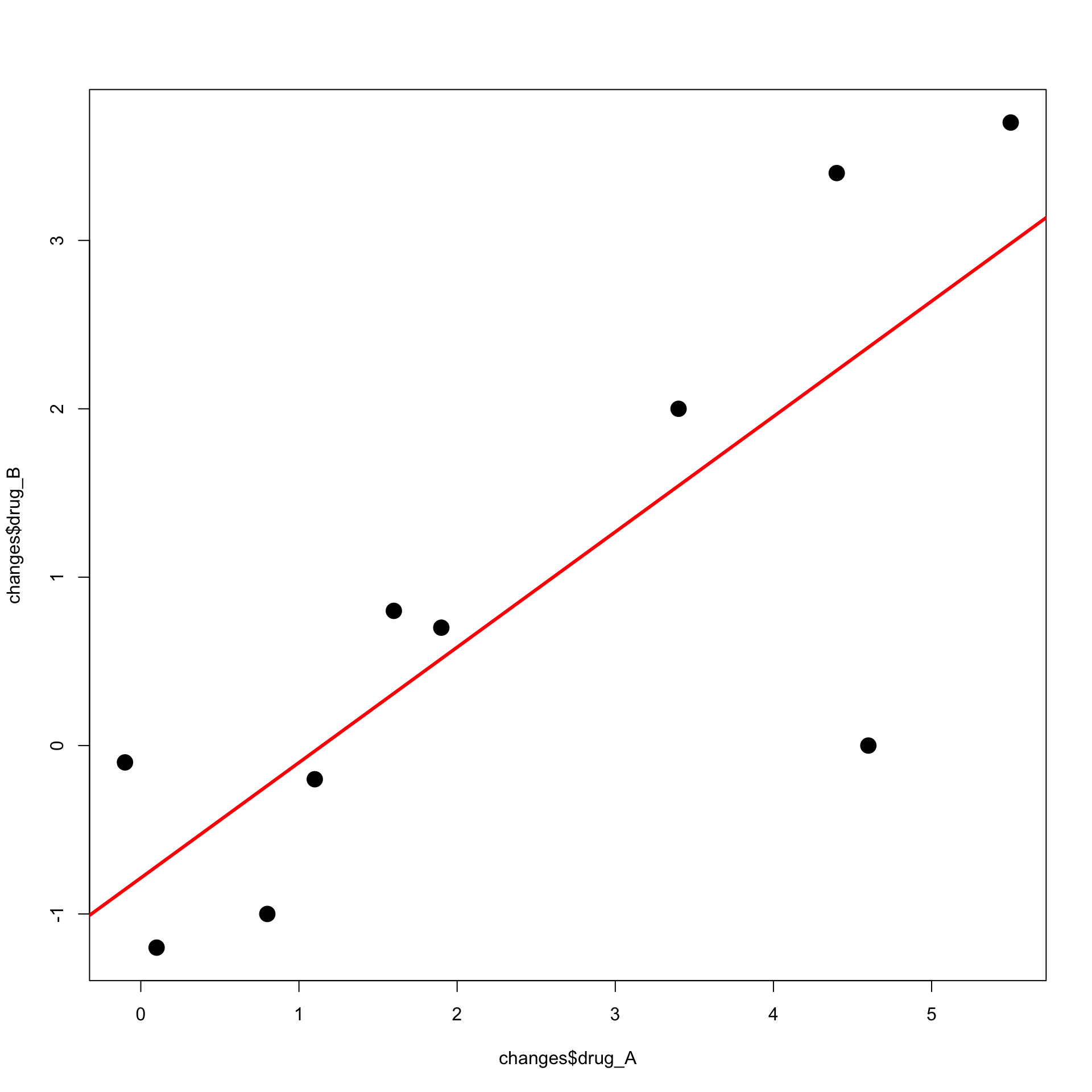
- Plot the data pairs (x_i,y_i)
# Plot the data
plot(x, y, xlab = "", ylab = "", pch = 16, cex = 2)

# Add labels
mtext("Drug A reaction x_i", side = 1, line = 3, cex = 2.1)
mtext("Drug B reaction y_i", side = 2, line = 2.5, cex = 2.1)- Note: We have added a few cosmetic options
pch = 16plots points with black circlescex = 2stands for character expansion – Specifies width of pointsxlab = ""andylab = ""add empty axis labels
Exercise: Blood Pressure
First Solution
- Plot the data pairs (x_i,y_i)
# Plot the data
plot(x, y, xlab = "", ylab = "", pch = 16, cex = 2)

# Add labels
mtext("Drug A reaction x_i", side = 1, line = 3, cex = 2.1)
mtext("Drug B reaction y_i", side = 2, line = 2.5, cex = 2.1)- Note: We have added a few cosmetic options
mtextis used to fine-tune the axis labelsside = 1stands for x-axisside = 2stands for y-axislinespecifies distance of label from axis
Exercise: Blood Pressure
First Solution
- To plot the least-squares line we need to
- Create grid of x coordinates and compute y = \hat \beta x + \hat \alpha over such grid
- Plot the pairs (x,y) and interpolate
# Compute least-squares line on grid
x_grid <- seq(from = -1, to = 6, by = 0.1)
y_grid <- beta * x_grid + alpha

# Plot the least-squares line
lines(x_grid, y_grid, col = "red", lwd = 3)- Note: Cosmetic options
colspecifies color of the plotlwdspecifies line width
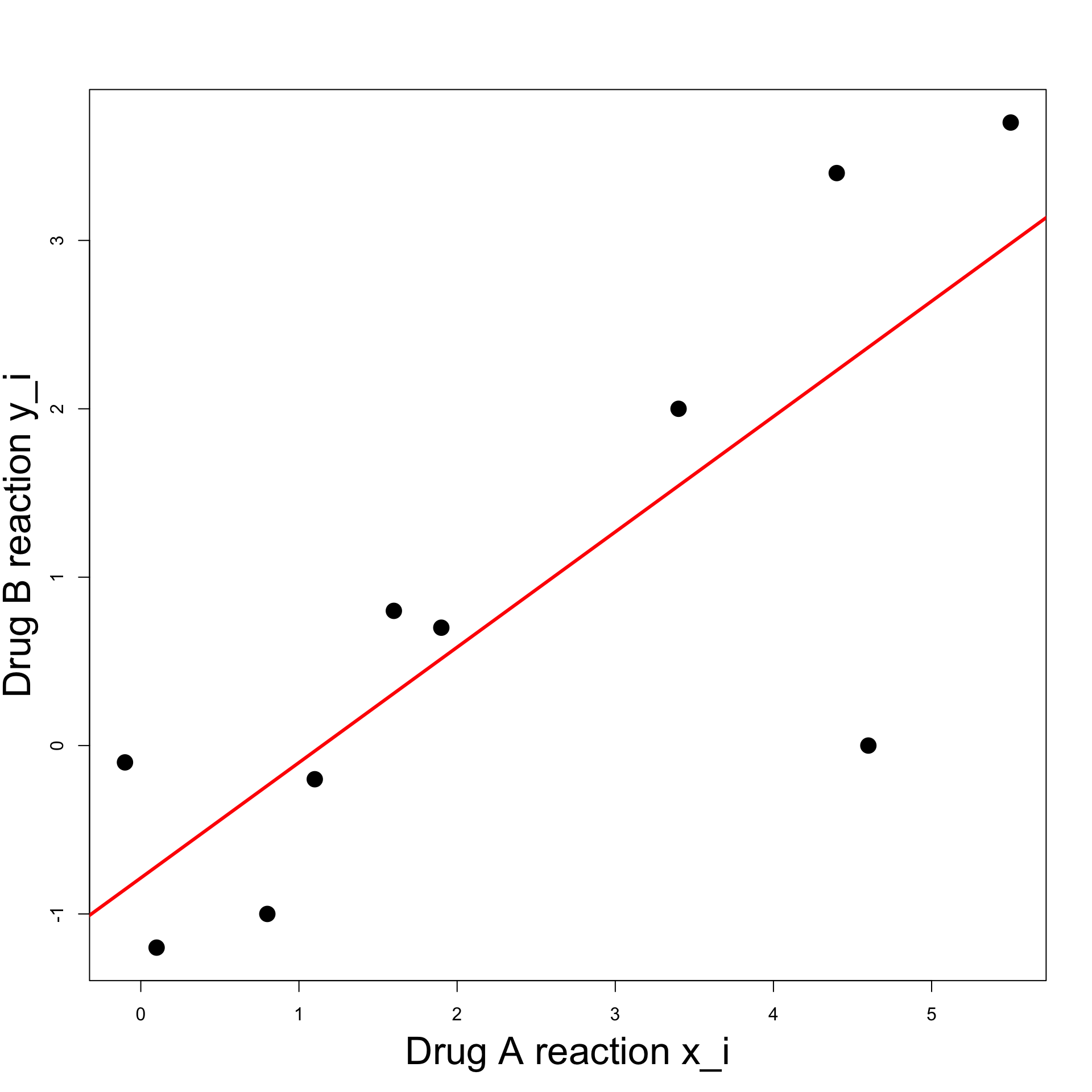
Exercise: Blood Pressure
First Solution
Previous code can be downloaded here least_squares_1.R
Running the code we obtain the plot on the right
Exercise: Blood Pressure
Second Solution
- The second solution uses the R function
lm lmstands for linear model- First we input the data into a data-frame
Exercise: Blood Pressure
Second Solution
We now use
lmto fit the least-squares lineThe basic syntax of
lmislm(formula, data)dataexpects a data-frame in inputformulastands for the relation to fit
In case of least-squares the formula is
formula = y ~ x
The symbol
y ~ xcan be read as- y modelled as function of x
xandyare the names of two variables in the data-frame
Exercise: Blood Pressure
Second Solution
- Storing data in data-frame is optional
- We can instead use vectors
xandy
- We can instead use vectors
- We can fit the least-squares line with command
lm(y ~ x)
Exercise: Blood Pressure
Second Solution
- The command to fit the least-squares line on
changesis
- This is what R plots when calling
print(least_squares)
Call:
lm(formula = drug_B ~ drug_A, data = changes)

Coefficients:
(Intercept)       drug_A
-0.7861 0.6850 - The above tells us that the estimators are
\hat \alpha = -0.7861 \,, \qquad \quad \hat \beta = 0.6850
Exercise: Blood Pressure
Second Solution
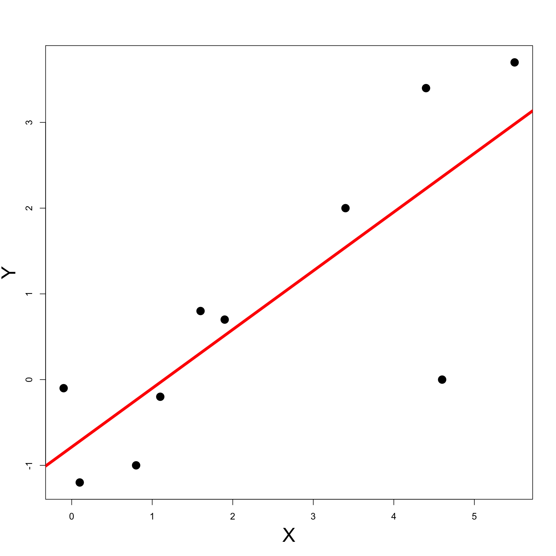
- We can now plot the data with the following command
- 1st coordinate is the vector
changes$drug_A - 2nd coordinate is the vector
changes$drug_B
- 1st coordinate is the vector
The least-squares line is currently stored in
least_squaresTo add such line to the current plot use
abline
Exercise: Blood Pressure
Second Solution
Previous code can be downloaded here least_squares_2.R
Running the code we obtain the plot on the right
Part 2:
Simple linear
regression
Simple linear regression
Motivation
- Model: Suppose to have two random variables X and Y
- X models observed values
- Y models a response
- Goal of Regression: Learn the distribution of
Y | X
- Y | X allows to predict values of Y from values of X
Simple linear regression
Motivation
Note: To learn Y|X one would need joint distribution of (X,Y)
Problem: The joint distribution of (X,Y) is unknown
Data: We have partial knowledge on (X,Y) in the form of
- paired observations (x_1,y_1) , \ldots, (x_n,y_n)
- (x_i,y_i) is observed from (X,Y)
Goal:Use the data to learn Y|X
Simple linear regression
Motivation
Least-Squares:
Naive solution to regression problem
Find a line of best fit y = \hat \alpha + \hat \beta x
Such line explains the data, i.e., y_i \ \approx \ \hat \alpha + \hat \beta x_i

Simple linear regression
Motivation
Drawbacks of least squares:
Only predicts values of y such that (x,y) \, \in \, \text{ Line}
Ignores that (x_i,y_i) comes from joint distribution (X,Y)
Simple linear regression
Motivation
Linear Regression:
Find a regression line R(x) = \alpha + \beta x
R(x) predicts most likely value of Y when X = x

Simple linear regression
Motivation
Linear Regression:
We will see that regression line coincides with line of best fit R(x) = \hat \alpha + \hat \beta x
Hence regression gives statistical meaning to the line of best fit

Regression function
Definition
Suppose given two random variables X and Y
- X is the predictor
- Y is the response
Definition
The regression function of Y on X is the conditional expectation
R \colon \mathbb{R}\to \mathbb{R}\,, \qquad \quad R(x) := {\rm I\kern-.3em E}[Y | X = x]
Regression function
Interpretation
Idea
The regression function
R(x) = {\rm I\kern-.3em E}[Y | X = x]
predicts the most likely value of Y when we observe
X = x
Notation: We use the shorthand {\rm I\kern-.3em E}[Y|x] := {\rm I\kern-.3em E}[Y | X = x]
The regression problem
Assumption: Suppose to have n observations (x_1,y_1) \,, \ldots , (x_n, y_n)
- x_i observed from X
- y_i observed from Y
Problem
From (x_1,y_1) \,, \ldots , (x_n, y_n) learn a regression function
{\rm I\kern-.3em E}[Y | x]
which explains the observations, that is,
{\rm I\kern-.3em E}[Y | x_i] \ \approx \ y_i \,, \qquad \forall \, i = 1 , \ldots, n
Simple linear regression
Regression problem is difficult without prior knowledge on {\rm I\kern-.3em E}[Y | x]
A popular model is to assume that {\rm I\kern-.3em E}[Y | x] is linear
Definition
The regression function of Y on X is linear if there exist \alpha and \beta s.t.
{\rm I\kern-.3em E}[Y | x] = \alpha + \beta x \,, \qquad \forall \, x \in \mathbb{R}
\alpha and \beta are called regression coefficients
The above regression is called simple because only 2 variables are involved
What do we mean by linear?
Note: We said that the regression is linear if {\rm I\kern-.3em E}[Y | x ] = \alpha + \beta x In the above we mean linearity wrt the parameters \alpha and \beta
Examples:
Linear regression of Y on X^2 is {\rm I\kern-.3em E}[Y | x^2 ] = \alpha + \beta x^2
Linear regression of \log Y on 1/X is {\rm I\kern-.3em E}[ \log Y | x ] = \alpha + \beta \frac{1}{ x }
Simple linear regression
Model Assumptions
Suppose to have n observations (x_1,y_1) \,, \ldots , (x_n, y_n)
- x_i observed from X
- y_i observed from Y
Definition
For each i = 1 , \ldots, n we denote by Y_i a random variable with distribution
Y | X = x_i
Assumptions:
- Predictor is known: The values x_1, \ldots, x_n are known
Simple linear regression
Model Assumptions
Normality: The distribution of Y_i is normal
Linear mean: There are parameters \alpha and \beta such that {\rm I\kern-.3em E}[Y_i] = \alpha + \beta x_i
Common variance (Homoscedasticity): There is a parameter \sigma^2 such that {\rm Var}[Y_i] = \sigma^2
Independence: The random variables Y_1 \,, \ldots \,, Y_n are independent
Characterization of the Model
- Assumptions 1–5 look quite abstract
- The following Proposition gives a handy characterization
Proposition
Assumptions 1-5 are satisfied if and only if
Y_i = \alpha + \beta x_i + \varepsilon_i
for some random variables
\varepsilon_1 , \ldots, \varepsilon_n \,\, \text{ iid } \,\, N(0,\sigma^2)
- The terms \varepsilon_i are called errors
Characterization of the Model
Proof
By Assumption 2 we have that Y_i is normal
By Assumption 3 and 4 we have
{\rm I\kern-.3em E}[Y_i] = \alpha + \beta x_i \,, \qquad \quad {\rm Var}[Y_i] = \sigma^2
- Therefore
Y_i \sim N(\alpha + \beta x_i, \sigma^2)
Characterization of the Model
Proof
- Define the random variables
\varepsilon_i := Y_i - (\alpha + \beta x_i)
By Assumption 5 we have that Y_1,\ldots,Y_n are independent
Therefore \varepsilon_1,\ldots,\varepsilon_n are independent
Since Y_i \sim N(\alpha + \beta x_i, \sigma^2) we conclude that
\varepsilon_i \sim N(0,\sigma^2)
Likelihood function
Definition
Let X_1, \ldots, X_n be continuous rv with joint pdf
f = f(x_1, \ldots, x_n | \theta)
depending on a parameter \theta \in \Theta. The likelihood function of the random vector (X_1, \ldots, X_n) for a given sample (x_1, \ldots, x_n) is
L \colon \Theta \to \mathbb{R}\,, \qquad \quad L(\theta | x_1,\ldots, x_n ) := f(x_1, \ldots, x_n | \theta)
Likelihood function
Proposition
Suppose Assumptions 1–5 hold. The likelihood function of linear regression is
L(\alpha,\beta, \sigma^2 | y_1, \ldots, y_n ) = \frac{1}{(2\pi \sigma^2)^{n/2}} \, \exp \left( -\frac{\sum_{i=1}^n(y_i-\alpha - \beta x_i)^2}{2\sigma^2} \right)
Likelihood function
Proof
- Recall that
Y_i \sim N( \alpha + \beta x_i , \sigma^2 )
- Therefore the pdf of Y_i is
f_{Y_i} (y_i) = \frac{1}{\sqrt{2\pi \sigma^2}} \exp \left( -\frac{(y_i-\alpha-\beta{x_i})^2}{2\sigma^2} \right)
Likelihood function
Proof
- Since Y_1,\ldots, Y_n are independent we obtain \begin{align*} L(\alpha,\beta, \sigma^2 | y_1, \ldots,y_n) & = f(y_1,\ldots,y_n) \\ & = \prod_{i=1}^n f_{Y_i}(y_i) \\ & = \prod_{i=1}^n \frac{1}{\sqrt{2\pi \sigma^2}} \exp \left( -\frac{(y_i-\alpha-\beta{x_i})^2}{2\sigma^2} \right) \\ & = \frac{1}{(2\pi \sigma^2)^{n/2}} \, \exp \left( -\frac{\sum_{i=1}^n(y_i- \alpha - \beta x_i)^2}{2\sigma^2} \right) \end{align*}
Model Summary
- Simple linear regression of Y on X is the function
{\rm I\kern-.3em E}[Y | x] = \alpha + \beta x
- Suppose given the observations from (X,Y)
(x_1,y_1) , \ldots , (x_n, y_n)
Model Summary
- Denote by Y_i the random variable
Y | X = x_i
- We suppose that Y_i has the form
Y_i = \alpha + \beta x_i + \varepsilon_i
- The errors \varepsilon_1,\ldots, \varepsilon_n are iid N(0,\sigma^2)
The linear regression problem
Problem
From (x_1,y_1) \,, \ldots , (x_n, y_n) learn a linear regression function
{\rm I\kern-.3em E}[Y | x] = \alpha + \beta x
which explains the observations, that is, \begin{equation} \tag{3}
{\rm I\kern-.3em E}[Y | x_i] \ \approx \ y_i \,, \qquad \forall \, i = 1 , \ldots, n
\end{equation}
Question
How do we enforce (3)?
Answer
- Recall that Y_i is distributed like
Y | x_i
- Therefore
{\rm I\kern-.3em E}[Y | x_i] = {\rm I\kern-.3em E}[Y_i]
- Hence (3) holds iff
\begin{equation} \tag{4} {\rm I\kern-.3em E}[Y_i] \ \approx \ y_i \,, \qquad \forall \, i = 1 , \ldots, n \end{equation}
Answer
- If we want (4) to hold, we need to maximize the joint probability
P(Y_1 \approx y_1, \ldots, Y_n \approx y_n)
- This means choosing parameters \hat \alpha, \hat \beta, \hat \sigma which maximize the likelihood function
\max_{\alpha,\beta,\sigma} \ L(\alpha,\beta, \sigma^2 | y_1, \ldots, y_n )
Maximizing the likelihood
Theorem
Suppose Assumptions 1–5 hold and assume given n observations (x_1,y_1), \ldots, (x_n,y_n). The maximization problem
\max_{\alpha,\beta,\sigma} \ L(\alpha,\beta, \sigma^2 | y_1, \ldots, y_n )
admits the unique solution
\hat \alpha = \overline{y} - \hat \beta \, \overline{x} \,, \qquad
\hat \beta = \frac{S_{xy}}{S_{xy}} \,, \qquad
\hat{\sigma}^2 = \frac{1}{n} \sum_{i=1}^n \left( y_i - \hat \alpha - \hat \beta x_i \right)^2
Note: The coefficients \hat \alpha and \hat \beta are the same of least-squares line!
Maximizing the likelihood
Proof of Theorem
The \log function is strictly increasing
Therefore the problem \max_{\alpha,\beta,\sigma} \ L(\alpha,\beta, \sigma^2 | y_1, \ldots, y_n ) is equivalent to \max_{\alpha,\beta,\sigma} \ \log L( \alpha,\beta, \sigma^2 | y_1, \ldots, y_n )
Maximizing the likelihood
Proof of Theorem
Recall that the likelihood is L(\alpha,\beta, \sigma^2 | y_1, \ldots, y_n ) = \frac{1}{(2\pi \sigma^2)^{n/2}} \, \exp \left( - \frac{\sum_{i=1}^n(y_i-\alpha - \beta x_i)^2}{2\sigma^2} \right)
Hence the log–likelihood is \log L(\alpha,\beta, \sigma^2 | y_1, \ldots, y_n ) = - \frac{n}{2} \log (2 \pi) - \frac{n}{2} \log \sigma^2 - \frac{ \sum_{i=1}^n(y_i-\alpha - \beta x_i)^2 }{2 \sigma^2}
Maximizing the likelihood
Proof of Theorem
Suppose \sigma is fixed. In this case the problem \max_{\alpha,\beta} \ \left\{ \frac{n}{2} \log (2 \pi) - \frac{n}{2} \log \sigma^2 - \frac{ \sum_{i=1}^n(y_i-\alpha - \beta x_i)^2 }{2 \sigma^2} \right\} is equivalent to \min_{\alpha, \beta} \ \sum_{i=1}^n(y_i-\alpha - \beta x_i)^2
This is the least-squares problem! Hence the solution is \hat \alpha = \overline{y} - \hat \beta \, \overline{x} \,, \qquad \hat \beta = \frac{S_{xy}}{S_{xy}}
Maximizing the likelihood
Proof of Theorem
Substituting \hat \alpha and \hat \beta we obtain \begin{align*} \max_{\alpha,\beta,\sigma} \ & \log L(\alpha,\beta, \sigma^2 | y_1, \ldots, y_n ) = \max_{\sigma} \ \log L(\hat \alpha, \hat \beta, \sigma^2 | y_1, \ldots, y_n ) \\[10pt] & = \max_{\sigma} \ \left\{ - \frac{n}{2} \log (2 \pi) - \frac{n}{2} \log \sigma^2 - \frac{ \sum_{i=1}^n(y_i-\hat\alpha - \hat\beta x_i)^2 }{2 \sigma^2} \right\} \end{align*}
It can be shown that the unique solution to the above problem is \hat{\sigma}^2 = \frac{1}{n} \sum_{i=1}^n \left( y_i - \hat \alpha - \hat \beta x_i \right)^2
This concludes the proof
Least-squares vs Linear regression
Linear regression and least-squares give seemingly the same answer
| Least-squares line | y = \hat \alpha + \hat \beta x |
|---|---|
| Linear regression line | {\rm I\kern-.3em E}[Y | x ] = \hat \alpha + \hat \beta x |
Question: Why did we define regression if it gives same answer as least-squares?
Least-squares vs Linear regression
Answer: There is actually a big difference
- Least-squares line y = \hat \alpha + \hat \beta x
- Just a geometric object
- Can only predict pairs (x,y) which lie on the line
- Ignores statistical nature of the problem
- Regression line {\rm I\kern-.3em E}[Y | x ] = \hat \alpha + \hat \beta x
- Statistical model for Y|X via the estimation of {\rm I\kern-.3em E}[Y | x]
- Can predict most likely values of Y given the observation X = x
- Can test how well the linear model fits the data
References
[1]
Fusco, Nicola, Marcellini, Paolo, Sbordone, Carlo, Mathematical analysis: Functions of several real variables and applications, Springer, 2022.