Statistical Models

Lecture 7

Dr. Silvio Fanzon

S.Fanzon@hull.ac.uk

University of Hull

Dr. John Fry

J.M.Fry@hull.ac.uk

University of Hull

Lecture 7:
The chi-squared test

Outline of Lecture 7

1. Overview
2. Chi-squared goodness-of-fit test
3. Goodness-of-fit test: Examples
4. Monte Carlo simulations
5. Contingency tables
6. Chi-squared test of independence
7. Test of independence: Examples

Part 1:
Overview

Problem statement

Data: in the form of numerical counts

Test: difference between observed counts and predictions of theoretical model

Example: Blood counts

• Suppose to have counts of blood type for some people

  A	B	AB	O
  2162	738	228	2876

• We want to compare the above to the probability model

  A	B	AB	O
  1/3	1/8	1/24	1/2

Counts with multiple factors

Manager	Won	Drawn	Lost
Moyes	27	9	15
Van Gaal	54	25	24
Mourinho	84	32	28
Solskjaer	91	37	40
Rangnick	11	10	8
ten Hag	61	12	28

Example: Relative performance of Manchester United managers

• Each football manager has Win, Draw and Loss count

Counts with multiple factors

Manager	Won	Drawn	Lost
Moyes	27	9	15
Van Gaal	54	25	24
Mourinho	84	32	28
Solskjaer	91	37	40
Rangnick	11	10	8
ten Hag	61	12	28

Questions:

• Is the number of Wins, Draws and Losses uniformly distributed?
• Are there differences between the performances of each manager?

Chi-squared test

• Hypothesis testing for counts can be done using chi-squared test

• Chi-squared test is simple to use for real-world project datasets (e.g. dissertations)

• Potentially applicable to a whole range of different models

• Easy to compute by hand/software

• Motivates the more advanced study of contingency tables

Part 2:
Chi-squared
goodness-of-fit test

Chi-squared goodness-of-fit test

Categorical Data:

• Finite number of possible categories or types
• Observations can only belong to one category
• O_i refers to observed count of category i

Type 1	Type 2	\ldots	Type n
O_1	O_2	\ldots	O_n

• E_i refers to expected count of category i

Type 1	Type 2	\ldots	Type n
E_1	E_2	\ldots	E_n

Chi-squared goodness of fit test

Goal: Compare expected counts E_i with observed counts O_i

Method:

• Null hypothesis: The theoretical model for expected counts is correct
• Look for evidence against the null hypothesis
• Null hypothesis is wrong
  • If distance between observed counts and expected counts is large
  • For example if (O_i - E_i)^2 \geq c for some chosen constant c

Chi-squared statistic

Definition

Global distance between observed and expected counts is defined as \chi^2 := \sum_{i=1}^n \frac{(O_i-E_i)^2}{E_i} The above is called chi-squared statistic

Note: We have that \chi^2 = 0 \qquad \iff \qquad O_i = E_i \,\,\,\, \text{ for all } \,\,\,\, i = 1 , \, \ldots , \, n

Chi-squared statistic

Remarks:

• We expect small differences between O_i and E_i
  • Therefore \chi^2 > 0
• However O_i should not be too far away from E_i
  • Therefore \chi^2 should not be too large
• The above imply that tests on \chi^2 should be one-sided

Modelling counts

Multinomial distribution: is a model for the following experiment

• The experiment consists of m independent trials
• Each trial results in one of n distinct possible outcomes
• The probability of the i-th outcome is p_i on every trial, with 0 \leq p_i \leq 1 \qquad \qquad \sum_{i=1}^n p_i = 1
• X_i counts the number of times i-th outcome occurred in the m trials. It holds \sum_{i=1}^n X_i = m

Modelling counts

Multinomial distribution: Schematic visualization

Outcome type	1	\ldots	n	Total
Counts	X_1	\ldots	X_n	X_1 + \ldots + X_n = m
Probabilities	p_1	\ldots	p_n	p_1 + \ldots + p_n = 1

Modelling counts

For n = 2 the multinomial reduces to a binomial:

• Each trial has n = 2 possible outcomes
• X_1 counts the number of successes
• X_2 = m − X_1 counts the number of failures in m trials
• Probability of success is p_1
• Probability of failure is p_2 = 1 - p_1

Outcome types	1	2
Counts	X_1	X_2 = m - X_1
Probabilities	p_1	p_2 = 1 - p_1

Multinomial distribution

Definition

Let m,n \in \mathbb{N} and p_1, \ldots, p_n numbers such that 0 \leq p_i \leq 1 \,, \qquad \quad \sum_{i=1}^n p_i = 1 The random vector \mathbf{X}= (X_1, \ldots, X_n) has multinomial distribution with m trials and cell probabilities p_1,\ldots,p_n if joint pmf if f (x_1, \ldots , x_n) = \frac{m!}{x_1 ! \cdot \ldots \cdot x_n !} \ p_1^{x_1} \cdot \ldots \cdot p_n^{x_n} \,, \qquad \forall \, x_i \in \mathbb{N}\, \, \text{ s.t. } \, \sum_{i=1}^n x_i = m We denote \mathbf{X}\sim \mathop{\mathrm{Mult}}(m,p_1,\ldots,p_n)

Multinomial distribution

Properties

Suppose that \mathbf{X}= (X_1, \ldots, X_n) \sim \mathop{\mathrm{Mult}}(m,p_1,\ldots,p_n)

• Then X_i is binomial with m trials and probability p_i
• We write X_i \sim \mathop{\mathrm{Bin}}(m,p_i) and the pmf is f(x_i) = P(X = x_i) = \frac{m!}{x_i! \cdot (1-x_i)!} \, p_i^{x_i} (1-p_i)^{1-x_i} \qquad \forall \, x_i = 0 , \ldots , m
• Since X_i \sim \mathop{\mathrm{Bin}}(m,p_i) it holds {\rm I\kern-.3em E}[X_i] = m p_i \qquad \qquad {\rm Var}[X_i] = m p_i (1-p_i)

Counts with Multinomial distribution

• O_i refers to observed count of category i

• E_i refers to expected count of category i

• We suppose that Type i is observed with probability p_i and 0 \leq p_i \leq 1 \,, \qquad \quad p_1 + \ldots + p_n = 1

• Total number of observations is m

• The counts are modelled by (O_1, \ldots, O_n) \sim \mathop{\mathrm{Mult}}(m, p_1, \ldots, p_n)

• The expected counts are modelled by E_i := {\rm I\kern-.3em E}[ O_i ] = m p_i

Counts with Multinomial distribution

Consider counts and expected counts (O_1, \ldots, O_n) \sim \mathop{\mathrm{Mult}}(m, p_1, \ldots, p_n) \qquad \qquad E_i := m p_i

Definition

The chi-squared statistic for multinomial counts is defined by \chi^2 = \sum_{i=1}^n \frac{(O_i-E_i)^2}{E_i} = \sum_{i=1}^n \frac{( O_i - m p_i )^2}{ m p_i }

Question: What is the distribution of \chi^2 \,?

Distribution of chi-squared statistic

Theorem

Suppose the counts (O_1, \ldots, O_n) \sim \mathop{\mathrm{Mult}}(m,p_1, \ldots, p_n). Then \chi^2 = \sum_{i=1}^n \frac{( O_i - m p_i )^2}{ m p_i } \ \stackrel{{\rm d}}{\longrightarrow} \ \chi_{n-1}^2 when sample size m \to \infty, where the convergence is in distribution

• Hence the distribution of \chi^2 is approximately \chi_{n-1}^2 when m is large

• The above Theorem is due to Karl Pearson in 1900 paper link

• Proof is difficult. Seven different proofs are presented in this paper link

Distribution of chi-squared statistic

Heuristic proof of Theorem

• Since O_i \sim \mathop{\mathrm{Bin}}(m, p_i), the Central Limit Theorem implies \frac{O_i - m p_i }{ \sqrt{m p_i(1 - p_i) } } \ \stackrel{{\rm d}}{\longrightarrow} \ N(0,1) as m \to \infty

• In particular, since (1-p_i) in constant, we have \frac{O_i - m p_i }{ \sqrt{m p_i } } \ \approx \ \frac{O_i - m p_i }{ \sqrt{m p_i(1 - p_i) } } \ \approx \ N(0,1)

Distribution of chi-squared statistic

Heuristic proof of Theorem

• Squaring the above we get \frac{(O_i - m p_i)^2 }{ m p_i } \ \approx \ N(0,1)^2 = \chi_1^2

• If the above random variables were pairwise independent, we would obtain \chi^2 = \sum_{i=1}^n \frac{(O_i - m p_i)^2 }{ m p_i } \ \approx \ \sum_{i=1}^n \chi_1^2 = \chi_n^2

• However the O_i are not independent because of linear constraint O_1 + \ldots + O_n = m

Distribution of chi-squared statistic

Heuristic proof of Theorem

• The idea is that a priori there should be n degrees of freedom

• However the linear constraint reduces degrees of freedom by 1

• This is because one can choose the first n-1 counts and the last one is given by O_n = m - O_1 - \ldots - O_{n-1}

• A rather technical proof is needed to actually prove that \chi^2 = \sum_{i=1}^n \frac{(O_i - m p_i)^2 }{ m p_i } \ \approx \ \chi_{n-1}^2

Quality of chi-squared approximation

• Define expected counts E_i := m p_i

• Consider approximation from Theorem: \chi^2 = \sum_{i=1}^n \frac{(O_i - E_i)^2 }{ E_i } \ \approx \ \chi_{n-1}^2

• The approximation is:

  Good	E_i \geq 5 \, \text{ for all } \, i = 1 , \ldots n
  Bad	E_i < 5 \, for some \, i = 1 , \ldots n

• Good: Use \chi_{n-1}^2 approximation of \chi^2

• Bad: Use Monte Carlo simulations (more on this later)

The chi-squared goodness-of-fit test

Setting:

• Population consists of items of n different types

• p_i is probability that an item selected at random is of type i

• p_i is unknown and needs to be estimated

• As guess for p_1,\ldots,p_n we take p_1^0, \ldots, p_n^0 such that 0 \leq p_i^0 \leq 1 \qquad \qquad \sum_{i=1}^n p_i^0 = 1

The chi-squared goodness-of-fit test

Hypothesis Test: We test for equality of p_i to p_i^0 \begin{align*} & H_0 \colon p_i = p_i^0 \qquad \text{ for all } \, i = 1, \ldots, n \\ & H_1 \colon p_i \neq p_i^0 \qquad \text{ for at least one } \, i \end{align*}

Sample:

• We draw m items from population
• O_i denotes the number of items of type i drawn
• Therefore (O_1, \ldots, O_n) \sim \mathop{\mathrm{Mult}}(m,p_1, \ldots, p_n)

The chi-squared goodness-of-fit test

Data: Vector of counts (o_1,\ldots,o_n)

Schematically: We can represent probabilities and counts in a table

Type	1	\ldots	n	Total
Counts	o_1	\ldots	o_n	m
Probabilities	p_1	\ldots	p_n	1

The chi-squared goodness-of-fit test

Procedure

1. Calculation:
   • Compute total counts and expected counts m = \sum_{i=1}^n o_i \qquad \quad E_i = m p_i^0
   • Compute the chi-squared statistic \chi^2 = \sum_{i=1}^n \frac{ (o_i - E_i)^2 }{E_i}

The chi-squared goodness-of-fit test

Procedure

2. Statistical Tables or R:
   • Check that E_i \geq 5 for all i = 1, \ldots, n
   • In this case \chi^2 \ \approx \ \chi_{n-1}^2
   • Find critical value in chi-squared Table 13.5 \chi^2_{n - 1} (0.05)
   • Alternatively, compute p-value in R p := P( \chi^2_{n - 1} > \chi^2 )

The chi-squared goodness-of-fit test

Procedure

3. Interpretation:
   • Reject H_0 if \chi^2 > \chi_{n - 1}^2 (0.05) \qquad \text{ or } \qquad p < 0.05
   • Do not reject H_0 if \chi^2 \leq \chi^2_{n - 1} (0.05) \qquad \text{ or } \qquad p \geq 0.05

The chi-squared goodness-of-fit test in R

General commands

1. Store the counts o_1,\ldots, o_n in R vector
   • counts <- c(o1, ..., on)
2. Store the null hypothesis probabilities p_1^0,\ldots, p_n^0 in R vector
   • null_probs <- c(p1, ..., pn)
3. Perform a goodness-of-fit test on counts with null_probs
   • chisq.test(counts, p = null_probs)
4. Read output
   • Output is similar to t-test and F-test
   • The main quantity of interest is p-value

Comments on chisq.test

1. R performs a goodness-of-fit test on counts with null_probs with

   • chisq.test(counts, p = null_probs)

2. R implicitly assumes the null hypothesis is H_0 \colon p_i = p_i^0 \qquad \text{ for all } \, i = 1 , \ldots, n

3. By default R computes p-value using \chi_{n-1}^2 approximation

4. R can compute p-value with Monte Carlo simulation using option

   • simulate.p.value = TRUE

Part 3:
Goodness-of-fit test:
Examples

Example: Blood counts

• Suppose to have counts of blood type for some people

  A	B	AB	O
  2162	738	228	2876

• We want to compare the above to the probability model

  A	B	AB	O
  1/3	1/8	1/24	1/2

• Hence the null hypothesis probabilities are p_1^0 = \frac{1}{3} \qquad \quad p_2^0 = \frac{1}{8} \qquad \quad p_3^0 = \frac{1}{24} \qquad \quad p_4^0 = \frac{1}{2}

Example: Blood counts

Goodness-of-fit test by hand

1. Calculation:
   • Compute total counts m = \sum_{i=1}^n o_i = 2162 + 738 + 228 + 2876 = 6004

Example: Blood counts

Goodness-of-fit test by hand

1. Calculation:
   • Compute expected counts \begin{align*} E_1 & = m p_1^0 = 6004 \times \frac{1}{3} = 2001.3 \\ E_2 & = m p_2^0 = 6004 \times \frac{1}{8} = 750.5 \\ E_3 & = m p_3^0 = 6004 \times \frac{1}{24} = 250.2 \\ E_4 & = m p_4^0 = 6004 \times \frac{1}{2} = 3002 \end{align*}

Example: Blood counts

Goodness-of-fit test by hand

1. Calculation:
   • Compute the chi-squared statistic \begin{align*} \chi^2 & = \sum_{i=1}^n \frac{ (o_i - E_i)^2 }{E_i} \\ & = \frac{ (2162 − 2001.3)^2 }{ 2001.3 } + \frac{ (738 − 750.5)^2 }{ 750.5 } \\ & \phantom{ = } + \frac{ (228 − 250.2)^2 }{ 250.2 } + \frac{ (2876 − 3002)^2 }{ 3002 } \\ & = 20.37 \end{align*}

Example: Blood counts

Goodness-of-fit test by hand

2. Statistical Tables:
   • Degrees of freedom are \, {\rm df} = n - 1 = 3
   • We have computed E_1 = 2001.3 \qquad E_2 = 750.5 \qquad E_3 = 250.2 \qquad E_4 = 3002
   • Hence E_i \geq 5 for all i = 1, \ldots, n
   • In this case \chi^2 \ \approx \ \chi_{3}^2
   • In chi-squared Table 13.5 we find critical value \chi^2_{3} (0.05) = 7.81

Example: Blood counts

Goodness-of-fit test by hand

3. Interpretation:
   • We have that \chi^2 = 20.37 > 7.81 = \chi_{3}^2 (0.05)
   • Therefore we reject H_0
4. Conclusion:
   • Observed counts suggest at least one of null probabilities p_i^0 is wrong

Example: Fair dice

Goodness-of-fit test in R

• A dice with 6 faces is rolled 100 times
• Counts observed are

1	2	3	4	5	6
13	17	9	17	18	26

• Exercise: Is the dice fair?
  • Formulate appropriate goodness-of-fit test
  • Implement this test in R

Example: Fair dice

Solution

• The dice is fair if probability of rolling i is 1/6
• Therefore we test the following hypothesis \begin{align*} & H_0 \colon p_i = \frac{1}{6} \qquad \text{ for all } \, i = 1, \ldots, n \\ & H_1 \colon p_i \neq \frac{1}{6} \qquad \text{ for at least one } \, i \end{align*}

Example: Fair dice

Solution

• Test can be performed using the code below
• Code can be downloaded here good_fit.R

# Enter counts and null hypothesis probabilities
counts <- c(13, 17, 9, 17, 18, 26)
null_probs <- rep(1/6, 6)

# Perform goodness-of-fit test
ans <- chisq.test(counts, p = null_probs)

# Print answer
print(ans)

Example: Fair dice

Solution

• Running the code in previous slide we obtain

    Chi-squared test for given probabilities

data:  counts
X-squared = 9.68, df = 5, p-value = 0.08483

• Chi-squared statistic is \, \chi^2 = 9.68

• Degrees of freedom are \, {\rm df} = 5

• p-value is p \approx 0.08

• Therefore p > 0.05

• We cannot reject H_0

• The dice appears to be fair

Example: Voting data

Goodness-of-fit test in R

• Assume there are two candidates: Republican and Democrat
• Voter can choose one of these or be undecided
• 100 people are surveyed and the results are

Republican	Democrat	Undecided
35	40	25

Example: Voting data

Goodness-of-fit test in R

• Hystorical data suggest that undecided voters are 30\% of population
• Exercise: Is difference between Republican and Democratic significant?
  • Formulate appropriate goodness-of-fit test
  • Implement this test in R
  • You are not allowed to use chisq.test

Example: Voting data

Solution

• Hystorical data suggest that undecided voters are 30\% of population
• Therefore we can assume that probability of undecided voter is p_3^0 = 0.3
• Want to test if there is difference between Republican and Democrat
• Hence null hypothesis is p_1^0 = p_2^0

Example: Voting data

Solution

• Recall that p_1^0 + p_2^0 + p_3^0 = 1

• Hence we deduce p_1^0 = 0.35 \qquad \quad p_2^0 = 0.35 \qquad \quad p_3^0 = 0.3

• We test the following hypothesis \begin{align*} & H_0 \colon p_i = p_i^0 \qquad \text{ for all } \, i = 1, \ldots, n \\ & H_1 \colon p_i \neq p_i^0 \qquad \text{ for at least one } \, i \end{align*}

Example: Voting data

Solution

• We want to perform goodness-of-fit test without using chisq.test

• First we enter the data

# Enter counts and null hypothesis probabilities
counts <- c(35, 40 , 25)
null_probs <- c(0.35, 0.35, 0.3)

Example: Voting data

Solution

• Compute the total number of counts m = o_1 + \ldots + o_n

# Compute total counts
m <- sum(counts)

• Compute degrees of freedom \, {\rm df} = n - 1

# Compute degrees of freedom
degrees <- length(counts) - 1

Example: Voting data

Solution

• Compute the expected counts E_i = m p_i^0

# Compute expected counts
exp_counts <- m * null_probs

• Compute chi-squared statistic \chi^2 = \sum_{i=1}^n \frac{( o_i - E_i )^2}{E_i}

# Compute chi-squared statistic
chi_squared <- sum( (counts - exp_counts)^2 / exp_counts )

Example: Voting data

Solution

• Finally compute the p-value p = P( \chi_{n-1}^2 > \chi^2 ) = 1 - P( \chi_{n-1}^2 \leq \chi^2 )

# Compute p-value
p_value <- 1 - pchisq(chi_squared, df = degrees)

# Print p-value
cat("The p-value is:", p_value)

• The full code can be downloaded here good_fit_first_principles.R

Example: Voting data

Solution

• Running the code gives the following output

The p-value is: 0.4612526

• Therefore p-value is p > 0.05

• We do not reject H_0

• There is no reason to believe that Republican and Democrat are not tie

Part 4:
Monte Carlo
simulations

Monte Carlo simulations

• Recall the approximation \chi^2 = \sum_{i=1}^n \frac{(O_i - E_i)^2 }{ E_i } \ \approx \ \chi_{n-1}^2

• We said that

  • E_i < 5 for some i \quad \implies \quad approximation of \chi^2 with \chi_{n-1}^2 is bad
  • In this case we use Monte Carlo simulations

• Question: What is a Monte Carlo simulation?

Monte Carlo methods

• Monte Carlo methods:
  • Broad class of computational algorithms
  • They rely on repeated random sampling to obtain numerical results
  • Principle: use randomness to solve problems which are deterministic
• Why the name?
  • Method was developed by Stanislaw Ulam
  • His uncle liked to gamble in the Monte–Carlo Casino in Monaco
• Examples of applications:
  • First used to solve problem of neutron diffusion in Los Alamos 1946
  • Can be used to compute p-values
  • Can be used to compute integrals

Monte Carlo simulation: Example

Approximating \pi

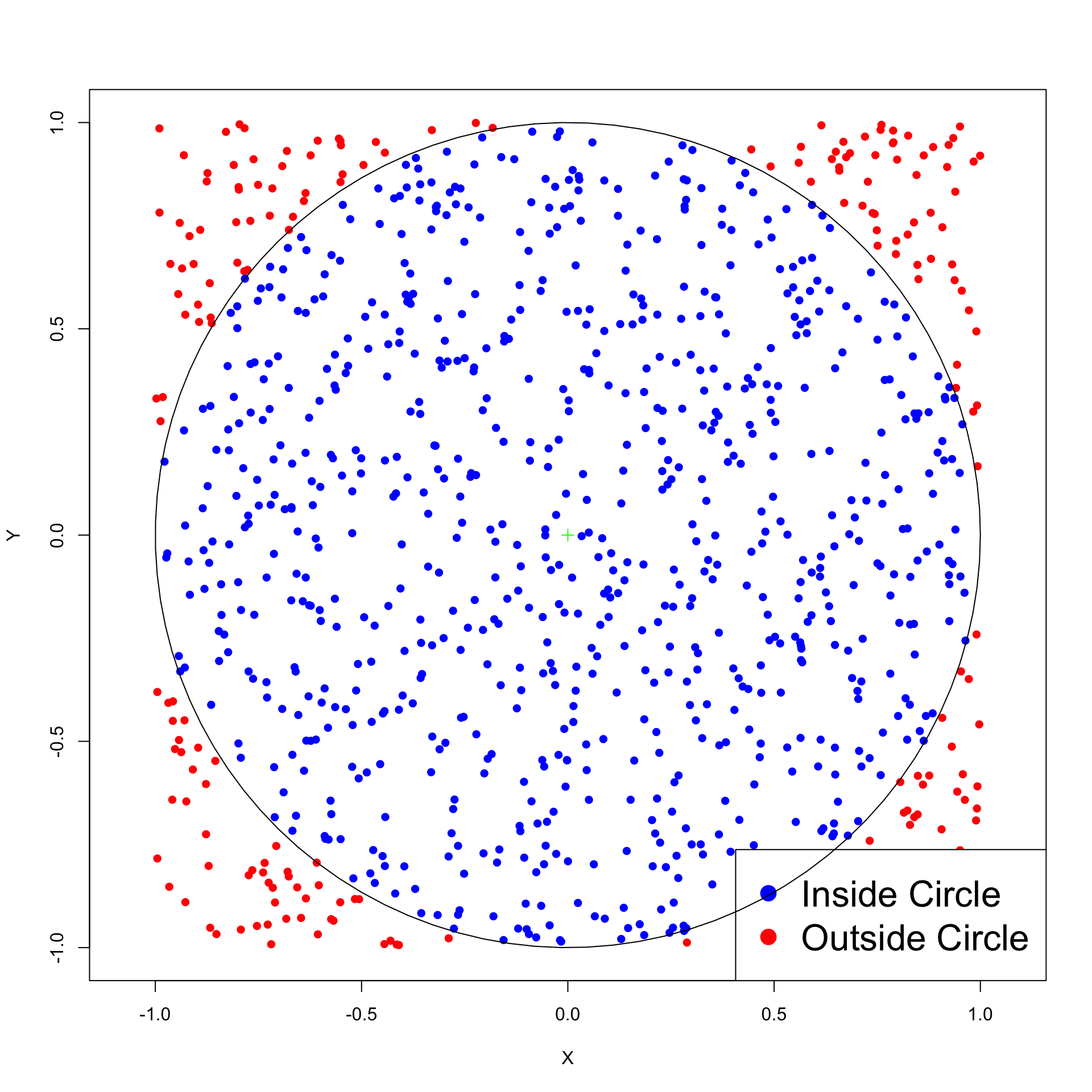
Monte Carlo simulation: Example

Approximating \pi – Summarizing the idea

• Throw random points inside square of side 2
• Count proportion of points falling inside unit circle
• Such proportion approximates the area of the circle
• Area of unit circle is \pi

Monte Carlo simulation: Example

Approximating \pi – Concrete steps

• Draw x_1, \ldots, x_N and y_1, \ldots, y_N from {\rm Uniform(-1,1)}

• Count the number of points (x_i,y_i) falling inside circle of radius 1

• These are points satisfying condition x_i^2 + y_i^2 \leq 1

• Area of circle estimated with proportion of points falling inside circle: \text{Area} \ = \ \pi \ \approx \ \frac{\text{Number of points } (x_i,y_i) \text{ inside circle}}{N} \ \times \ 4

• Note: 4 is the area of square of side 2

Monte Carlo simulation: Example

Plot of 1000 random points in square of side 2

Monte Carlo simulation: Example

Implementation in R – Download code monte_carlo_pi.R

N <- 10000
total <- 0      # Counts total number of points
in_circle <- 0  # Counts points falling in circle

for (j in 1:10) {
  for (i in 1:N) {
    x <- runif(1, -1, 1); y <- runif(1, -1, 1);  # sample point (x,y)
    if (x^2 + y^2 <= 1) {    
      in_circle <- in_circle + 1  # If (x,y) in circle increase counter
    }
    total <- total + 1  # Increase total counter
  }
  
  pi_approx <- ( in_circle / total ) * 4  # Compute approximate area

  cat(sprintf("After %8d iterations pi is %.08f, error is %.08f\n",
     (j * N), pi_approx, abs(pi_approx - pi)))
}

Monte Carlo simulation: Example

Implementation in R: Output

After    10000 iterations pi is 3.15480000, error is 0.01320735
After    20000 iterations pi is 3.15240000, error is 0.01080735
After    30000 iterations pi is 3.14320000, error is 0.00160735
After    40000 iterations pi is 3.14230000, error is 0.00070735
After    50000 iterations pi is 3.14432000, error is 0.00272735
After    60000 iterations pi is 3.14553333, error is 0.00394068
After    70000 iterations pi is 3.15017143, error is 0.00857877
After    80000 iterations pi is 3.15190000, error is 0.01030735
After    90000 iterations pi is 3.15004444, error is 0.00845179
After   100000 iterations pi is 3.14744000, error is 0.00584735

Monte Carlo p-value

Goal: use Monte Carlo simulations to compute p-value of goodness-of-fit test

• Consider data counts

Type	1	\ldots	n	Total
Observed counts	o_1	\ldots	o_n	m
Null hypothesis Probabilities	p_1^0	\ldots	p_n^0	1

• The expected counts are E_i = m p_i^0

• Under the null hypothesis, the observed counts (o_1, \ldots, o_n) come from (O_1 , \ldots, O_n) \sim \mathop{\mathrm{Mult}}(m, p_1^0, \ldots, p_n^0)

Monte Carlo p-value

• The chi-squared statistic random variable is \chi^2 = \sum_{i=1}^n \frac{(O_i - E_i)^2 }{ E_i }

• The observed chi-squared statistics is \chi^2_{\rm obs} = \sum_{i=1}^n \frac{(o_i - E_i)^2 }{ E_i }

• The p-value is defined as p = P( \chi^2 > \chi^2_{\rm obs} )

Monte Carlo p-value

Problem

• Suppose E_i < 5 for some i
• Then the distribution of chi-squared random variable is unknown \chi^2 = \sum_{i=1}^n \frac{(O_i - E_i)^2 }{ E_i } \ \, \sim \ \, ???
• How do we compute the p-value p = P( \chi^2 > \chi^2_{\rm obs} ) \ \ ???

Exercise: Think of Monte Carlo simulation to approximate p

Monte Carlo p-value

Solution

1. Simulate counts (o_1^{\rm sim},\ldots,o_n^{\rm sim}) from \mathop{\mathrm{Mult}}(m, p_1^0, \ldots, p_n^0)

2. Compute the corresponding simulated chi-squared statistic \chi^2_{\rm sim} = \sum_{i=1}^n \frac{ (o_i^{\rm sim} - E_i)^2 }{E_i}

3. The simulated chi-squared statistic is extreme if \, \chi^2_{\rm sim} > \chi^2_{\rm obs}

4. We estimate theoretical p-value in the following way p = P( \chi^2 > \chi^2_{\rm obs} ) \ \approx \ \frac{ \# \text{ of extreme simulated statistics} }{ \text{Total number of simulations} }

Monte Carlo p-value

Exercise

Data: Number of defects in printed circuit boards

# Defects	0	1	2	3
Counts	32	15	9	4

Null hypothesis probabilities are

p_1^0	p_2^0	p_3^0	p_4^0
0.5	0.3	0.15	0.05

Monte Carlo p-value

Exercise

• Total number of counts is m = 60. Expected counts are E_i = m p_i^0

E_1	E_2	E_3	E_4
30	18	9	3

• Note: E_4 = 3 < 5
  • Therefore the distribution of \chi^2 is unknown
• Exercise: Write an R code for goodness-of-fit test on above data
  • You may not use the function chisq.test
  • p-value should be computed by Monte Carlo simulations
  • Use the ideas in Slide 60

Monte Carlo p-value

Solution

• The first part of the code is the same as in Slides 44–46
  • Enter observed counts and null probabilities
  • Compute total counts, expected counts and observed chi-squared statistic

# Enter counts and null hypothesis probabilities
counts <- c(32, 15, 9, 4)
null_probs <- c(0.5, 0.3, 0.15, 0.05)

# Compute total counts
m <- sum(counts)

# Compute expected counts
exp_counts <- m * null_probs

# Compute the observed chi-squared statistic
obs_chi_squared <- sum( (counts - exp_counts)^2 / exp_counts )

Monte Carlo p-value

Solution

• We approximate the p-value using ideas in Slide 60
• We perform N Monte Carlo simulations

# Number of Monte Carlo simulations
N <- 100000

• To count extreme statistics we initialize a counter

# Initialize counter for extreme statistics
count_extreme_statistics <- 0

Monte Carlo p-value

Solution

• For each simulation we do
  • Simulate counts (o_1^{\rm sim},\ldots,o_n^{\rm sim}) from \mathop{\mathrm{Mult}}(m, p_1^0, \ldots, p_n^0)
  • Compute the corresponding simulated chi-squared statistic \chi^2_{\rm sim} = \sum_{i=1}^n \frac{ (o_i^{\rm sim} - E_i)^2 }{E_i}
  • Check if simulated statistic \chi^2_{\rm sim} is extreme, that is, if \chi^2_{\rm sim} > \chi^2_{\rm obs}
  • If \chi^2_{\rm sim} is extreme we increase the counter

Monte Carlo p-value

Solution

• The procedure discussed in the previous slide is coded below

# Perform Monte Carlo simulations

for (i in 1:N) {
  # Simulate multinomial counts under null hypothesis
  simul_counts <- rmultinom(1, m, null_probs)
  
  # Compute chi-squared statistic for the simulated counts
  simul_chi_squared <- sum( (simul_counts - exp_counts )^2 / exp_counts)
  
  # Check if simulated chi-squared statistic is extreme
  if (simul_chi_squared >= obs_chi_squared) {
    count_extreme_statistics <- count_extreme_statistics + 1
  }
}

Monte Carlo p-value

Solution

• We compute the Monte Carlo p-value using the below formula p \ = \ \frac{ \# \text{ of extreme simulated statistics} }{ \text{Total number of simulations} }

# Compute Monte Carlo p-value
monte_carlo_p_value <- count_extreme_statistics / N

Monte Carlo p-value

Solution

• To check our procedure we also compute Monte-Carlo p-value with chisq.test

# Perform chi-squared test using built-in R function
chi_squared_test <- chisq.test(counts, p = null_probs, 
                               simulate.p.value = TRUE)

# Extract p-value from chi-squared test result
chisq_p_value <- chi_squared_test$p.value

# Print p-values for comparison
cat("\nCustom Monte Carlo p-value:", monte_carlo_p_value)
cat("\nR Monte Carlo p-value:", chisq_p_value)

Monte Carlo p-value

Solution

• The previous code can be downloaded here monte_carlo_p_value.R

• Running the code yields the following output

Custom Monte Carlo p-value: 0.81921

R Monte Carlo p-value: 0.816092

• Notes:
  • chisq.test runs a more refined Monte Carlo algorithm for p-value
  • Even if our algorithm is quite elementary, the two p-values are close!
  • In particular p > 0.05 and we do not reject H_0

Part 5:
Contingency tables

Contingency tables: Example

Two-way Contigency Tables: Table in which each observation is classified in 2 ways

Example: Relative performance of Man Utd managers

• Two classifications for each game: Result and Manager in charge

Manager	Won	Drawn	Lost
Moyes	27	9	15
Van Gaal	54	25	24
Mourinho	84	32	28
Solskjaer	91	37	40
Rangnick	11	10	8
ten Hag	61	12	28

Contingency tables: General case

	Y = 1	Y = 2	\ldots	Y = C	Totals
X = 1	O_{11}	O_{12}	\ldots	O_{1C}	O_{1+}
X = 2	O_{21}	O_{22}	\ldots	O_{2C}	O_{2+}
\cdots	\cdots	\cdots	\ldots	\cdots	\cdots
X = R	O_{R1}	O_{R2}	\ldots	O_{RC}	O_{R+}
Totals	O_{+1}	O_{+2}	\ldots	O_{+C}	m

• Each observation
  • has attached two categories X and Y
  • can only belong to one category (X,Y) = (i,j)
• O_{ij} is the count of observations with (X,Y) = (i,j)
• Table has R rows and C columns for total of n = RC categories

Contingency tables: General case

	Y = 1	Y = 2	\ldots	Y = C	Totals
X = 1	O_{11}	O_{12}	\ldots	O_{1C}	O_{1+}
X = 2	O_{21}	O_{22}	\ldots	O_{2C}	O_{2+}
\cdots	\cdots	\cdots	\ldots	\cdots	\cdots
X = R	O_{R1}	O_{R2}	\ldots	O_{RC}	O_{R+}
Totals	O_{+1}	O_{+2}	\ldots	O_{+C}	m

• plus symbol in subscript denotes sum over that subscript. Example

O_{R+} = \sum_{j=1}^C O_{Rj} \qquad \quad O_{+2} = \sum_{i=1}^R O_{i2}

Contingency tables: General case

	Y = 1	Y = 2	\ldots	Y = C	Totals
X = 1	O_{11}	O_{12}	\ldots	O_{1C}	O_{1+}
X = 2	O_{21}	O_{22}	\ldots	O_{2C}	O_{2+}
\cdots	\cdots	\cdots	\ldots	\cdots	\cdots
X = R	O_{R1}	O_{R2}	\ldots	O_{RC}	O_{R+}
Totals	O_{+1}	O_{+2}	\ldots	O_{+C}	m

• The total count is

m = O_{++} = \sum_{i=1}^R \sum_{j=1}^C O_{ij}

Contingency tables: General case

	Y = 1	Y = 2	\ldots	Y = C	Totals
X = 1	O_{11}	O_{12}	\ldots	O_{1C}	O_{1+}
X = 2	O_{21}	O_{22}	\ldots	O_{2C}	O_{2+}
\cdots	\cdots	\cdots	\ldots	\cdots	\cdots
X = R	O_{R1}	O_{R2}	\ldots	O_{RC}	O_{R+}
Totals	O_{+1}	O_{+2}	\ldots	O_{+C}	m

• The marginal counts sum to m as well

\sum_{i=1}^R O_{i+} = \sum_{i=1}^R \sum_{j=1}^C O_{ij} = m

Contingency tables: General case

	Y = 1	Y = 2	\ldots	Y = C	Totals
X = 1	O_{11}	O_{12}	\ldots	O_{1C}	O_{1+}
X = 2	O_{21}	O_{22}	\ldots	O_{2C}	O_{2+}
\cdots	\cdots	\cdots	\ldots	\cdots	\cdots
X = R	O_{R1}	O_{R2}	\ldots	O_{RC}	O_{R+}
Totals	O_{+1}	O_{+2}	\ldots	O_{+C}	m

• The marginal counts sum to m as well

\sum_{j=1}^C O_{+j} = \sum_{j=1}^C \sum_{i=1}^R O_{ij} = m

Contingency tables: Probabilities

	Y = 1	Y = 2	\ldots	Y = C	Totals
X = 1	p_{11}	p_{12}	\ldots	p_{1C}	p_{1+}
X = 2	p_{21}	p_{22}	\ldots	p_{2C}	p_{2+}
\cdots	\cdots	\cdots	\ldots	\cdots	\cdots
X = R	p_{R1}	p_{R2}	\ldots	p_{RC}	p_{R+}
Totals	p_{+1}	p_{+2}	\ldots	p_{+C}	1

• Observation in cell (i,j) happens with probability

p_{ij} := P(X = i , Y = j)

Contingency tables: Probabilities

	Y = 1	Y = 2	\ldots	Y = C	Totals
X = 1	p_{11}	p_{12}	\ldots	p_{1C}	p_{1+}
X = 2	p_{21}	p_{22}	\ldots	p_{2C}	p_{2+}
\cdots	\cdots	\cdots	\ldots	\cdots	\cdots
X = R	p_{R1}	p_{R2}	\ldots	p_{RC}	p_{R+}
Totals	p_{+1}	p_{+2}	\ldots	p_{+C}	1

• The marginal probabilities that X = i or Y = j are at the margins of table

P(X = i) = \sum_{j=1}^C P(X = i , Y = j) = \sum_{j=1}^C p_{ij} = p_{i+}

Contingency tables: Probabilities

	Y = 1	Y = 2	\ldots	Y = C	Totals
X = 1	p_{11}	p_{12}	\ldots	p_{1C}	p_{1+}
X = 2	p_{21}	p_{22}	\ldots	p_{2C}	p_{2+}
\cdots	\cdots	\cdots	\ldots	\cdots	\cdots
X = R	p_{R1}	p_{R2}	\ldots	p_{RC}	p_{R+}
Totals	p_{+1}	p_{+2}	\ldots	p_{+C}	1

• The marginal probabilities that X = i or Y = j are at the margins of table

P(Y = j) = \sum_{i=1}^R P(X = i , Y = j) = \sum_{i=1}^R p_{ij} = p_{+j}

Contingency tables: Probabilities

	Y = 1	Y = 2	\ldots	Y = C	Totals
X = 1	p_{11}	p_{12}	\ldots	p_{1C}	p_{1+}
X = 2	p_{21}	p_{22}	\ldots	p_{2C}	p_{2+}
\cdots	\cdots	\cdots	\ldots	\cdots	\cdots
X = R	p_{R1}	p_{R2}	\ldots	p_{RC}	p_{R+}
Totals	p_{+1}	p_{+2}	\ldots	p_{+C}	1

• Marginal probabilities sum to 1

\sum_{i=1}^R p_{i+} = \sum_{i=1}^R P(X = i) = \sum_{i=1}^R \sum_{j=1}^C P(X = i , Y = j) = 1

Contingency tables: Probabilities

	Y = 1	Y = 2	\ldots	Y = C	Totals
X = 1	p_{11}	p_{12}	\ldots	p_{1C}	p_{1+}
X = 2	p_{21}	p_{22}	\ldots	p_{2C}	p_{2+}
\cdots	\cdots	\cdots	\ldots	\cdots	\cdots
X = R	p_{R1}	p_{R2}	\ldots	p_{RC}	p_{R+}
Totals	p_{+1}	p_{+2}	\ldots	p_{+C}	1

• Marginal probabilities sum to 1

\sum_{j=1}^C p_{+j} = \sum_{j=1}^C P(X = j) = \sum_{j=1}^R \sum_{j=1}^C P(X = i , Y = j) = 1

Multinomial distribution

• Counts O_{ij} and probabilities p_{ij} can be assembled into R \times C matrices O = \left( \begin{array}{ccc} O_{11} & \ldots & O_{1C} \\ \vdots & \ddots & \vdots \\ O_{R1} & \ldots & O_{RC} \\ \end{array} \right) \qquad \qquad p = \left( \begin{array}{ccc} p_{11} & \ldots & p_{1C} \\ \vdots & \ddots & \vdots \\ p_{R1} & \ldots & p_{RC} \\ \end{array} \right)

• This way the random matrix O has multinomial distribution O \sim \mathop{\mathrm{Mult}}(m,p)

• The counts O_{ij} are therefore binomial O_{ij} \sim \mathop{\mathrm{Bin}}(m,p_{ij})

Multinomial distribution

• We can also consider the marginal random vectors (O_{1+}, \ldots, O_{R+}) \qquad \qquad (O_{+1}, \ldots, O_{+C})

• These have also multinomial distribution (O_{1+}, \ldots, O_{R+}) \sim \mathop{\mathrm{Mult}}(m, p_{1+}, \ldots, p_{R+}) (O_{+1}, \ldots, O_{+C}) \sim \mathop{\mathrm{Mult}}(m, p_{+1}, \ldots, p_{+C})

Expected counts

	Y = 1	Y = 2	\ldots	Y = C	Totals
X = 1	O_{11}	O_{12}	\ldots	O_{1C}	O_{1+}
X = 2	O_{21}	O_{22}	\ldots	O_{2C}	O_{2+}
\cdots	\cdots	\cdots	\ldots	\cdots	\cdots
X = R	O_{R1}	O_{R2}	\ldots	O_{RC}	O_{R+}
Totals	O_{+1}	O_{+2}	\ldots	O_{+C}	m

• We have that O_{ij} \sim \mathop{\mathrm{Bin}}(m,p_{ij})
• Therefore we model the expected counts for category (i,j) as E_{ij} := {\rm I\kern-.3em E}[O_{ij}] = m p_{ij}

Marginal expected counts

	Y = 1	Y = 2	\ldots	Y = C	Totals
X = 1	E_{11}	E_{12}	\ldots	E_{1C}	E_{1+}
X = 2	E_{21}	E_{22}	\ldots	E_{2C}	E_{2+}
\cdots	\cdots	\cdots	\ldots	\cdots	\cdots
X = R	E_{R1}	E_{R2}	\ldots	E_{RC}	E_{R+}
Totals	E_{+1}	E_{+2}	\ldots	E_{+C}	m

• Due to linearity of expectation, it makes sense to define marginal counts E_{i+} := \sum_{j=1}^C E_{ij} \qquad \qquad E_{+j} := \sum_{i=1}^R E_{ij}

Marginal expected counts

	Y = 1	Y = 2	\ldots	Y = C	Totals
X = 1	E_{11}	E_{12}	\ldots	E_{1C}	E_{1+}
X = 2	E_{21}	E_{22}	\ldots	E_{2C}	E_{2+}
\cdots	\cdots	\cdots	\ldots	\cdots	\cdots
X = R	E_{R1}	E_{R2}	\ldots	E_{RC}	E_{R+}
Totals	E_{+1}	E_{+2}	\ldots	E_{+C}	m

• Marginal expected counts sum to m. For example: \sum_{i=1}^R E_{i+} = \sum_{i=1}^R \sum_{j=1}^C E_{ij} = m \sum_{i=1}^R \sum_{j=1}^C p_{ij} = m

The chi-squared statistic

	Y = 1	Y = 2	\ldots	Y = C	Totals
X = 1	O_{11}	O_{12}	\ldots	O_{1C}	O_{1+}
X = 2	O_{21}	O_{22}	\ldots	O_{2C}	O_{2+}
\cdots	\cdots	\cdots	\ldots	\cdots	\cdots
X = R	O_{R1}	O_{R2}	\ldots	O_{RC}	O_{R+}
Totals	O_{+1}	O_{+2}	\ldots	O_{+C}	m

Definition

The chi-squared statistic associated to the above contingency table is \chi^2 := \sum_{i=1}^R \sum_{j=1}^C \frac{ (O_{ij} - E_{ij})^2 }{ E_{ij} } = \sum_{i=1}^R \sum_{j=1}^C \frac{ (O_{ij} - m p_{ij})^2 }{ m p_{ij} }

Distribution of chi-squared statistic

Theorem

Suppose the counts O \sim \mathop{\mathrm{Mult}}(m,p). Then \chi^2 = \sum_{i=1}^R \sum_{j=1}^C \frac{ (O_{ij} - m p_{ij})^2 }{ m p_{ij} } \ \stackrel{ {\rm d} }{ \longrightarrow } \ \chi_{RC - 1 - {\rm fitted} }^2 when sample size m \to \infty. The convergence is in distribution and

• \rm fitted = \, # of parameters used to estimate cell probabilities p_{ij}

Quality of approximation: The chi-squared approximation is good if E_{ij} = m p_{ij} \geq 5 \quad \text{ for all } \,\, i = 1 , \ldots , R \, \text{ and } j = 1, \ldots, C

Goodness-of-fit test for contingency tables

Setting:

• Population consists of items of n = R \times C different types

• p_{ij} is probability that an item selected at random is of type (i,j)

• p_{ij} is unknown and needs to be estimated

• As guess for p_{ij} we take p_{ij}^0 such that 0 \leq p_{ij}^0 \leq 1 \qquad \qquad \sum_{i=1}^R \sum_{j=1}^C p_{ij}^0 = 1

Goodness-of-fit test for contingency tables

Hypothesis Test: We test for equality of p_{ij} to p_{ij}^0 \begin{align*} & H_0 \colon p_{ij} = p_{ij}^0 \qquad \text{ for all } \, i = 1, \ldots, R \,, \text{ and } \, j = 1 , \ldots, C \\ & H_1 \colon p_{ij} \neq p_{ij}^0 \qquad \text{ for at least one pair } \, (i,j) \end{align*}

Sample:

• We draw m items from population
• O_{ij} denotes the number of items of type i drawn
• Therefore O = (O_{ij})_{ij} is \mathop{\mathrm{Mult}}(m,p) with p = (p_{ij})_{ij}

Data: Matrix of counts o = (o_{ij})_{ij}

Goodness-of-fit test for contingency tables

Procedure

1. Calculation:
   • Compute total counts and expected counts m = \sum_{i=1}^R \sum_{j=1}^C o_{ij} \qquad \quad E_{ij} = m p_{ij}^0
   • Compute the chi-squared statistic \chi^2 = \sum_{i=1}^R \sum_{j=1}^C \frac{ (o_{ij} - E_{ij})^2 }{E_{ij}}

Goodness-of-fit test for contingency tables

Procedure

2. Statistical Tables or R:
   • Check that E_{ij} \geq 5 for all i, j
   • We did not fit any parameter. Hence the Theorem in Slide 88 gives {\rm degrees \,\, freedom} = RC - 1 \qquad \qquad \chi^2 \ \approx \ \chi_{RC-1}^2
   • Find critical value in chi-squared Table 13.5 \chi^2_{RC - 1} (0.05)
   • Alternatively, compute p-value in R p := P( \chi^2_{RC - 1} > \chi^2 )

Goodness-of-fit test for contingency tables

Procedure

3. Interpretation:
   • Reject H_0 if \chi^2 > \chi_{RC - 1}^2 (0.05) \qquad \text{ or } \qquad p < 0.05
   • Do not reject H_0 if \chi^2 \leq \chi^2_{RC - 1} (0.05) \qquad \text{ or } \qquad p \geq 0.05

Goodness-of-fit test in R

General commands

1. Store the matrix of counts O = (o_{ij})_{ij} into a single R vector, proceeding row-by-row
   • counts <- c(o_11, o_12, ..., o_RC)
2. Store the matrix of null probabilities p = (p_{ij})_{ij} into a single R vector, proceeding row-by-row
   • null_probs_i <- c(p_11, p_12, ..., p_RC)
3. Perform a chi-squared goodness-of-fit test on counts with null_probs
   • chisq.test(counts, p = null_probs)
4. Read output: In particular look for the p-value

Note: Compute Monte Carlo p-value with option simulate.p.value = TRUE

Example: Manchester United performance

Background story:

• From 1992 to 2013 Man Utd won 13 Premier Leagues out of 21
• This is the best performance in the Premier League era
• This was under manager Sir Alex Ferguson
• Ferguson stepped down in 2014
• Since 2014 Man Utd has not won the PL and was managed by 6 different people (excluding interims)

Question: Are the 6 managers to blame for worse Team Performance?

Example: Manchester United performance

Manager	Won	Drawn	Lost
Moyes	27	9	15
Van Gaal	54	25	24
Mourinho	84	32	28
Solskjaer	91	37	40
Rangnick	11	10	8
ten Hag	61	12	28

• Table contains Man Utd games since 2014 season

• To each Man Utd game in the sample we associate two categories:

  • Manager and Result

Example: Manchester United performance

• Question: Is the number of Wins, Draws and Losses uniformly distributed?

  • If Yes, this would suggest very poor performance

• Hypothesis Test: To answer the question we perform a goodness-of-fit test on \begin{align*} & H_0 \colon p_{ij} = p_{ij}^0 \quad \text { for all pairs } \, (i,j) \\ & H_1 \colon p_{ij} \neq p_{ij}^0 \quad \text { for at least one pair } \, (i,j) \\ \end{align*}

• Null Probabilities:

  • They have to model that Wins, Draws and Losses are uniformly distributed
  • To compute them, we need to compute total number of games for each manager

Example: Manchester United performance

• We compute total number of games for each manager

Manager	Won	Drawn	Lost	Total
Moyes	27	9	15	o_{1+} = 51
Van Gaal	54	25	24	o_{2+} = 103
Mourinho	84	32	28	o_{3+} = 144
Solskjaer	91	37	40	o_{4+} = 168
Rangnick	11	10	8	o_{5+} = 29
ten Hag	61	12	28	o_{6+} = 101

• We also need the total number of games m = \sum_{i=1}^R o_{i+} = 596

Example: Manchester United performance

• If the results are uniformly distributed the expected scores are E_{ij} = \frac{o_{i+}}{3}

• Recall that the expected scores are modelled as E_{ij} = m p_{ij}^0

• We hence obtain p_{ij}^0 = \frac{o_{i+}}{3 m}

Example: Manchester United performance

• Substituting the values of o_{i+} and m we finally obtain the null probabilities

\begin{align*} \text{Moyes: } \quad & p_{1j}^0 = \frac{ o_{1+} }{ 3m } = 51 \big/ 1788 \\ \text{Van Gaal: }\quad & p_{2j}^0 = \frac{ o_{2+} }{ 3m } = 103 \big/ 1788 \\ \text{Mourinho: } \quad& p_{3j}^0 = \frac{ o_{3+} }{ 3m } = 144 \big/ 1788 \\ \text{Solskjaer: } \quad& p_{4j}^0 = \frac{ o_{4+} }{ 3m } = 168 \big/ 1788 \\ \text{Rangnick: }\quad & p_{5j}^0 = \frac{ o_{5+} }{ 3m } = 29 \big/ 1788 \\ \text{ten Hag: }\quad & p_{6j}^0 = \frac{ o_{6+} }{ 3m } = 101 \big/ 1788 \end{align*}

Example: Manchester United performance

• We are now ready to perform the goodness-of-fit test in R

• We start by storing the matrix of counts into a single R vector, row-by-row

# Store matrix of counts into single R vector
counts <- c(27, 9, 15,
            54, 25, 24,
            84, 32, 28, 
            91, 37, 40,
            11, 10, 8,
            61, 12, 28)

Example: Manchester United performance

• Then we store the matrix of null probabilities into a single R vector, row-by-row
• Null probabilities in each row are the same. Hence we can use the command rep

# Store matrix of null probabilities into single R vector
# We use repeat to avoid copy pasting 
lines_null_probs <- c(51/1788, 103/1788, 144/1788, 
                      168/1788, 29/1788, 101/1788)

null_probs <- rep(lines_null_probs, c(3, 3, 3, 3, 3, 3))

Example: Manchester United performance

• Finally we perform the goodness-of-fit test on counts and null_probs

# Perform goodness-of-fit test
ans <- chisq.test(counts, p = null_probs)

# Print answer
print(ans)

• The code can be downloaded here good_fit_contingency.R

Example: Manchester United performance

• Running the code we obtain

    Chi-squared test for given probabilities

data:  counts
X-squared = 137.93, df = 17, p-value < 2.2e-16

• p-value is p \approx 0 < 0.05
• We therefore reject H_0
• Significant evidence that results of Man Utd games are not uniformly distributed
• Low goal-scoring rates in soccer mean roughly 1/3 of games end in a draw
• Hence Man Utd is not actually doing too bad

Part 6:
Chi-squared test
of independence

Testing for independence

	Owned	Rented	Total
North West	2180	871	3051
London	1820	1400	3220
South West	1703	614	2317
Total	5703	2885	8588

• Consider a two-way contingency table as above

• To each person we associate two categories:

  • Residential Status: Rental or Owned
  • Region in which they live: NW, London, SW

Testing for independence

	Owned	Rented	Total
North West	2180	871	3051
London	1820	1400	3220
South West	1703	614	2317
Total	5703	2885	8588

• One possible question is:
  • Does Residential Status depend on Region?
  • In other words: Are rows and columns dependent?

Testing for independence

	Owned	Rented	Total
North West	2180	871	3051
London	1820	1400	3220
South West	1703	614	2317
Total	5703	2885	8588

• Looking at the data, it seems clear that:
  • London: Rentals are almost comparable to Owned
  • NW and SW: Rentals are almost a third of Owned
  • It appears Residential Status and Region are dependent features
• Goal: Formulate test for independence

Testing for independence

	Y = 1	\ldots	Y = C	Totals
X = 1	O_{11}	\ldots	O_{1C}	O_{1+}
\cdots	\cdots	\cdots	\cdots	\cdots
X = R	O_{R1}	\ldots	O_{RC}	O_{R+}
Totals	O_{+1}	\ldots	O_{+C}	m

• Consider the general two-way contingency table as above

• They are equivalent:

  • Rows and columns are independent
  • Random variables X and Y are independent

Testing for independence

	Y = 1	\ldots	Y = C	Totals
X = 1	O_{11}	\ldots	O_{1C}	O_{1+}
\cdots	\cdots	\cdots	\cdots	\cdots
X = R	O_{R1}	\ldots	O_{RC}	O_{R+}
Totals	O_{+1}	\ldots	O_{+C}	m

• Hence, testing for independece means testing following hypothesis: \begin{align*} & H_0 \colon X \, \text{ and } \, Y \, \text{ are independent } \\ & H_1 \colon X \, \text{ and } \, Y \, \text{ are not independent } \end{align*}

• We need to quantify H_0 and H_1

Testing for independence

	Y = 1	\ldots	Y = C	Totals
X = 1	p_{11}	\ldots	p_{1C}	p_{1+}
\cdots	\cdots	\cdots	\cdots	\cdots
X = R	p_{R1}	\ldots	p_{RC}	p_{R+}
Totals	p_{+1}	\ldots	p_{+C}	1

• R.v. X and Y are independent iff cell probabilities factor into marginals p_{ij} = P(X = i , Y = j) = P(X = i) P (Y = j) = p_{i+}p_{+j}

• Therefore the hypothesis test for independence becomes \begin{align*} & H_0 \colon p_{ij} = p_{i+}p_{+j} \quad \text{ for all } \, i = 1, \ldots , R \, \text{ and } \, j = 1 ,\ldots C \\ & H_1 \colon p_{ij} \neq p_{i+}p_{+j} \quad \text{ for some } \, (i,j) \end{align*}

Expected counts

• Assume the null hypothesis is true H_0 \colon p_{ij} = p_{i+}p_{+j} \quad \text{ for all } \, i = 1, \ldots , R \, \text{ and } \, j = 1 ,\ldots C

• Under H_0 the expected counts become E_{ij} = m p_{ij} = p_{i+}p_{+j}

• We need a way to estimate the marginal probabilities p_{i+} and p_{+j}

Estimating marginal probabilities

• Goal: Estimate marginal probabilities p_{i+} and p_{+j}

• By definition we have p_{i+} = P( X = i )

• Hence p_{i+} is probability of and observation to be classified in i-th row

• Estimate p_{i+} with the proportion of observations classified in i-th row p_{i+} := \frac{o_{i+}}{m} = \frac{ \text{Number of observations in } \, i\text{-th row} }{ \text{ Total number of observations} }

Estimating marginal probabilities

• Goal: Estimate marginal probabilities p_{i+} and p_{+j}

• Similarly, by definition p_{+j} = P( Y = j )

• Hence p_{+j} is probability of and observation to be classified in j-th column

• Estimate p_{+j} with the proportion of observations classified in j-th column p_{+j} := \frac{o_{+j}}{m} = \frac{ \text{Number of observations in } \, j\text{-th column} }{ \text{ Total number of observations} }

\chi^2 statistic for testing independence

• Summary: The marginal probabilities are estimated with p_{i+} := \frac{o_{i+}}{m} \qquad \qquad p_{+j} := \frac{o_{+j}}{m}

• Therefore the expected counts become E_{ij} = m p_{ij} = m p_{i+} p_{+j} = m \left( \frac{o_{i+}}{m} \right) \left( \frac{o_{+j}}{m} \right) = \frac{o_{i+} \, o_{+j}}{m}

• By the Theorem in Slide 88 the chi-squared statistics satisfies \chi^2 = \sum_{i=1}^R \sum_{j=1}^C \frac{ (O_{ij} - E_{ij})^2 }{ E_{ij} } \ \approx \ \chi^2_{RC - 1 - {\rm fitted}}

• We need to compute the number of fitted parameters

Number of fitted parameters

• We have to estimate the row marginals p_{i+}

• We estimate the first R-1 row marginals by p_{i+} := \frac{o_{i+}}{m} \,, \qquad i = 1 , \ldots, R - 1

• Since the marginals p_{i+} sum to 1, we can obtain p_{R+} by p_{R+} = 1 - p_{1+} - \ldots - p_{(R-1)+} = 1 - \frac{o_{1+}}{m} - \ldots - \frac{o_{(R-1)+}}{m}

Number of fitted parameters

• Similarly, we estimate the first C-1 column marginals by p_{+j} = \frac{o_{+j}}{m} \,, \qquad j = 1, \ldots, C - 1

• Since the marginals p_{+j} sum to 1, we can obtain p_{+C} by p_{+C} = 1 - p_{+1} - \ldots - p_{+(C-1)} = 1 - \frac{o_{+1}}{m} - \ldots - \frac{o_{+(C-1)}}{m}

• In total we only have to estimate (R - 1) + (C - 1 ) = R + C - 2 parameters

Number of fitted parameters

• In total we estimate R + C -2 parameters, so that {\rm fitted} = R + C - 2

• Therefore the degrees of freedom are \begin{align*} RC - 1 - {\rm fitted} & = RC - 1 - R - C + 2 \\ & = RC - R - C + 1 \\ & = (R - 1)(C - 1) \end{align*}

\chi^2 statistic for testing independence

Conclusion

• Assume the null hypothesis of row and column independence H_0 \colon p_{ij} = p_{i+}p_{+j} \quad \text{ for all } \, i = 1, \ldots , R \, \text{ and } \, j = 1 ,\ldots C

• Suppose the counts are O \sim \mathop{\mathrm{Mult}}(m,p) and expected counts are E_{ij} = \frac{o_{i+} \, o_{+j}}{m}

• By the previous slides and Theorem in Slide 88 we have that \chi^2 = \sum_{i=1}^R \sum_{j=1}^C \frac{ (O_{ij} - E_{ij})^2 }{ E_{ij} } \approx \ \chi_{RC - 1 - {\rm fitted} }^2 = \chi_{(R-1)(C-1)}^2

\chi^2 statistic for testing independence

Quality of approximation

The chi-squared approximation \chi^2 = \sum_{i=1}^R \sum_{j=1}^C \frac{ (O_{ij} - E_{ij})^2 }{ E_{ij} } \approx \ \chi_{(R-1)(C-1)}^2 is good if E_{ij} \geq 5 \quad \text{ for all } \,\, i = 1 , \ldots , R \, \text{ and } j = 1, \ldots, C

The chi-squared test of independence

Sample:

• We draw m items from population

• Each item can be of type (i,j) where

  • i = 1 , \ldots ,R
  • j = 1 , \ldots ,C
  • Total of n = RC types

• O_{ij} denotes the number of items of type (i,j) drawn

• p_{ij} is probability of observing type (i,j)

• p = (p_{ij})_{ij} is probability matrix

• The matrix of counts O = (o_{ij})_{ij} has multinomial distribution \mathop{\mathrm{Mult}}(m,p)

The chi-squared test of independence

Data: Matrix of counts, represented by two-way contigency table

	Y = 1	\ldots	Y = C	Totals
X = 1	o_{11}	\ldots	o_{1C}	o_{1+}
\cdots	\cdots	\cdots	\cdots	\cdots
X = R	o_{R1}	\ldots	o_{RC}	o_{R+}
Totals	o_{+1}	\ldots	o_{+C}	m

Hypothesis test: We test for independence of rows and columns \begin{align*} & H_0 \colon X \, \text{ and } \, Y \, \text{ are independent } \\ & H_1 \colon X \, \text{ and } \, Y \, \text{ are not independent } \end{align*}

The chi-squared test of independence

Procedure

1. Calculation:
   • Compute total counts m = \sum_{i=1}^R \sum_{j=1}^C o_{ij}
   • Compute marginal counts o_{i+} := \sum_{j=1}^C o_{ij} \qquad \qquad o_{+j} := \sum_{i=1}^R o_{ij}

The chi-squared test of independence

Procedure

1. Calculation:
   • Compute estimated expected counts E_{ij} = \frac{o_{i+} \, o_{+j} }{ m }
   • Compute the chi-squared statistic \chi^2 = \sum_{i=1}^R \sum_{j=1}^C \frac{ (o_{ij} - E_{ij})^2 }{E_{ij}}

The chi-squared test of independence

Procedure

2. Statistical Tables or R:
   • Check that E_{ij} \geq 5 for all i and j
   • In this case \chi^2 \ \approx \ \chi_{(R-1)(C-1)}^2
   • Find critical value in chi-squared Table 13.5 \chi^2_{(R-1)(C-1)} (0.05)
   • Alternatively, compute p-value in R p := P( \chi^2_{(R-1)(C-1)} > \chi^2 )

The chi-squared test of independence

Procedure

3. Interpretation:
   • Reject H_0 if \chi^2 > \chi_{(R-1)(C-1)}^2 (0.05) \qquad \text{ or } \qquad p < 0.05
   • Do not reject H_0 if \chi^2 \leq \chi^2_{(R-1)(C-1)} (0.05) \qquad \text{ or } \qquad p \geq 0.05

The chi-squared test of independence in R

General commands

1. Store each row of counts (o_{i1}, o_{i2}, \ldots, o_{iC}) in R vector
   • row_i <- c(o_i1, o_i2, ..., o_iC)
2. Assemble the rows into an R matrix
   • counts <- rbind(row_1, ..., row_R)
   • counts models the matrix of counts o = (o_{ij})_{ij}
3. Perform a chi-squared test of independence on counts
   • chisq.test(counts)
4. Read output: In particular look for the p-value

Note: Compute Monte Carlo p-value with option simulate.p.value = TRUE

Part 7:
Test of independence:
Examples

Example: Residential Status and Region

	Owned	Rented	Total
North West	2180	871	3051
London	1820	1400	3220
South West	1703	614	2317
Total	5703	2885	8588

• People are sampled at random in NW, London and SW

• To each person we associate two categories:

  • Residential Status: Rental or Owned
  • Region in which they live: NW, London, SW

• Exercise: Test for independence of Residential Status and Region

Example: Residential Status and Region

Chi-squared test of independence by hand

1. Calculation:
   • Rows are R = 3 and columns are C = 2
   • Total and marginal counts are already provided in the table

	Owned	Rented	Tot
NW	2180	871	o_{1+} = 3051
Lon	1820	1400	o_{2+} = 3220
SW	1703	614	o_{2+} = 2317
Tot	o_{+1} = 5703	o_{+2} = 2885	m = 8588

Example: Residential Status and Region

Chi-squared test of independence by hand

1. Calculation:
   • Compute the estimated expected counts E_{ij} = \dfrac{o_{i+} \, o_{+j} }{ m }

	Owned	Rented	Tot
NW	\frac{3051{\times}5703}{8588} \approx 2026	\frac{3051{\times}2885}{8588} \approx 1025	o_{1+} = 3051
Lon	\frac{3220{\times}5703}{8588} \approx 2138	\frac{3220{\times}2885}{8588} \approx 1082	o_{2+} = 3220
SW	\frac{2317{\times}5703}{8588} \approx 1539	\frac{2317{\times}1885}{8588} \approx 778	o_{2+} = 2317
Tot	o_{+1} = 5703	o_{+2} = 2885	m = 8588

Example: Residential Status and Region

Chi-squared test of independence by hand

1. Calculation:
   • Compute the chi-squared statistic \begin{align*} \chi^2 & = \sum_{i=1}^R \sum_{j=1}^C \frac{ (o_{ij} - E_{ij})^2 }{E_{ij}} \\ & = \frac{(2180-2026.066)^2}{2026.066} + \frac{(871-1024.934)^2}{1024.934} \\ & \, + \frac{(1820-2138.293)^2}{2138.293}+\frac{(1400-1081.707)^2}{1081.707} \\ & \, + \frac{(1703-1538.641)^2}{1538.641}+\frac{(614-778.359)^2}{778.359} \\ \end{align*}

Example: Residential Status and Region

Chi-squared test of independence by hand

1. Calculation:
   • Compute the chi-squared statistic \begin{align*} \chi^2 & = \sum_{i=1}^R \sum_{j=1}^C \frac{ (o_{ij} - E_{ij})^2 }{E_{ij}} \\ & = 11.695+23.119 \\ & \, + 47.379+93.658 \\ & \, + 17.557+34.707 \\ & = 228.12 \qquad (2\ \text{d.p.}) \end{align*}

Example: Residential Status and Region

Chi-squared test of independence by hand

2. Statistical Tables:
   • Degrees of freedom are \, {\rm df} = (R - 1)(C - 1) = 2
   • We clearly have E_{ij} \geq 5 for all i and j
   • Therefore the following approximation holds \chi^2 \ \approx \ \chi_{(R - 1)(C - 1)}^2 = \chi_{2}^2
   • In chi-squared Table 13.5 we find critical value \chi^2_{2} (0.05) = 5.99

Example: Residential Status and Region

Chi-squared test of independence by hand

3. Interpretation:
   • We have that \chi^2 = 228.12 > 5.99 = \chi_{2}^2 (0.05)
   • Therefore we rejct H_0, meaning that rows and columns are dependent

Example: Residential Status and Region

Chi-squared test of independence by hand

4. Conclusion:

• There is evidence (p < 0.05) that Residential Status depends on Region
• By rescaling table values, we can compute the table of percentages

	Owned	Rented
North West	71.5\%	28.5\%
London	56.5\%	43.5\%
South West	73.5\%	26.5\%

• The above suggests that in London fewer homes are Owned and more Rented

Example: Residential Status and Region

Chi-squared test of independence in R

• Test can be performed using code independence_test.R

# Store each row into and R vector
row_1 <- c(2180, 871)
row_2 <- c(1820, 1400)
row_3 <- c(1703, 614)

# Assemble the rows into an R matrix
counts <- rbind(row_1, row_2, row_3)

# Perform chi-squared test of independence
ans <- chisq.test(counts)

# Print answer
print(ans)

Example: Residential Status and Region

Chi-squared test of independence in R

• Running the code we obtain

    Pearson's Chi-squared test

data:  counts
X-squared = 228.11, df = 2, p-value < 2.2e-16

• This confirms the chi-squared statistic computed by hand \chi^2 = 228.11
• It also confirms the degrees of freedom \, {\rm df} = 2
• The p-value is p \approx 0 < 0.05
• Therefore H_0 is rejected and Residential Status depends on Region

Example: Manchester United performance

Recap of Background story:

• From 1992 to 2013 Man Utd won 13 Premier Leagues out of 21
• This is the best performance in the Premier League era
• This was under manager Sir Alex Ferguson
• Ferguson stepped down in 2014
• Since 2014 Man Utd has not won the PL and was managed by 6 different people (excluding interims)

Question: Are the 6 managers to blame for worse Team Performance?

Example: Manchester United performance

Manager	Won	Drawn	Lost
Moyes	27	9	15
Van Gaal	54	25	24
Mourinho	84	32	28
Solskjaer	91	37	40
Rangnick	11	10	8
ten Hag	61	12	28

• Table contains Man Utd games since 2014 season

• To each Man Utd game in the sample we associate two categories:

  • Manager and Result

• Question: Is there association between Manager and Team Performance?

Example: Manchester United performance

• To answer the question we perform chi-square test of independence in R

• Test can be performed by suitably modifying the code independence_test.R

# Store each row into and R vector
row_1 <- c(27, 9, 15)
row_2 <- c(54, 25, 24) 
row_3 <- c(84, 32, 28) 
row_4 <- c(91, 37, 40)
row_5 <- c(11, 10, 8)
row_6 <- c(61, 12, 28)

# Assemble the rows into an R matrix
counts <- rbind(row_1, row_2, row_3, row_4, row_5, row_6)

# Perform chi-squared test of independence
ans <- chisq.test(counts)

# Print answer
print(ans)

Example: Manchester United performance

Chi-squared test of independence in R

• Running the code we obtain

    Pearson's Chi-squared test

data:  counts
X-squared = 12.678, df = 10, p-value = 0.2422

• p-value is p \approx 0.24 > 0.05
• We do not reject H_0
• There is no evidence of association between Manager and Team Performance
• This suggests that there are deep structural problems that cannot be resolved simply by changing the Manager