Statistical Models

Lecture 6

Dr. Silvio Fanzon

S.Fanzon@hull.ac.uk

University of Hull

Dr. John Fry

J.M.Fry@hull.ac.uk

University of Hull

Lecture 6:
Two-sample
hypothesis tests

Outline of Lecture 6

Two-sample hypothesis tests
Two-sample t-test
Two-sample t-test: Example
Two-sample F-test
Two-sample F-test: Example

Part 1:
Two-sample
hypothesis tests

Overview

In Lecture 4:

Looked at data before and after the 2008 crash
In this case data for each month is directly comparable
Can then construct the difference between the 2007 and 2009 values
Analysis reduces from a two-sample to a one-sample problem

Question

How do we analyze two samples that cannot be paired?

Problem statement

Goal: compare mean and variance of 2 independent samples

First sample:
- Sample size n, sample mean \overline{x}, sample variance s^2_X
Second sample:
- Sample size m, sample mean \overline{y}, sample variance s^2_Y
We may have n \neq m
- Samples cannot be paired!

Tests available:

Two-sample t-test to test for difference in means
Two-sample F-test to test for difference in variances

Why is this important?

Hypothesis testing starts to get interesting with 2 or more samples
t-test and F-test show the normal distribution family in action
This is also the maths behind regression
- Same methods apply to seemingly unrelated problems
- Regression is a big subject in statistics

Normal distribution family in action

Two-sample t-test

Want to compare the means of two independent samples
At the same time population variances are unknown
Therefore both variances are estimated with sample variances
Test statistic is t_k-distributed with k linked to the total number of observations

Normal distribution family in action

Two-sample F-test

Want to compare the variance of two independent samples
This can be done by studying the ratio of the sample variances s^2_X/s^2_Y
We have already shown that \frac{(n - 1) S^2_X}{\sigma^2_X} \sim \chi^2_{n - 1} \qquad \frac{(m - 1) S^2_Y}{\sigma^2_Y} \sim \chi^2_{m - 1}

Normal distribution family in action

Two-sample F-test

Hence we can study statistic F = \frac{S^2_X / \sigma_X^2}{S^2_Y / \sigma_Y^2}
We will see that F has F-distribution

Part 2:
Two-sample t-test

The two-sample t-test

Assumptions: Suppose given samples from 2 normal populations

X_1, \ldots ,X_n iid with distribution N(\mu_X,\sigma^2)
Y_1, \ldots ,Y_m iid with distribution N(\mu_Y,\sigma^2)

Further assumptions:

In general n \neq m so that one-sample t-test cannot be applied
The two populations have same variance \sigma^2_X = \sigma^2_Y = \sigma^2

Note: Assuming same variance is simplification. Removing it leads to Welch t-test

The two-sample t-test

Goal: Compare means \mu_X and \mu_Y. We consider test H_0 \colon \mu_X = \mu_Y \qquad H_1 \colon \mu_X \neq \mu_Y

t-statistic: The general form is T = \frac{\text{Estimate}-\text{Hypothesised value}}{\text{e.s.e.}}

The two-sample t-statistic

Define the sample means \overline{X} = \frac{1}{n} \sum_{i=1}^n X_i \qquad \qquad \overline{Y} = \frac{1}{m} \sum_{i=1}^m Y_i
Notice that {\rm I\kern-.3em E}[ \overline{X} ] = \mu_X \qquad \qquad {\rm I\kern-.3em E}[ \overline{Y} ] = \mu_Y
Therefore we can estimate \mu_X - \mu_Y with the sample means, that is, \text{Estimate} = \overline{X} - \overline{Y}

The two-sample t-statistic

Since we are testing for difference in mean, we have \text{Hypothesised value} = \mu_X - \mu_Y
The Estimated Standard Error is the standard deviation of estimator \text{e.s.e.} = \text{Standard Deviation of } \overline{X} -\overline{Y}

The two-sample t-statistic

Therefore the two-sample t-statistic is T = \frac{\overline{X} - \overline{Y} - (\mu_X - \mu_Y)}{\text{e.s.e.}}
Under the Null Hypothesis that \mu_X = \mu_Y the t-statistic becomes T = \frac{\overline{X} - \overline{Y} }{\text{e.s.e.}}

A note on the degrees of freedom (df)

The general rule is \text{df} = \text{Sample size} - \text{No. of estimated parameters}
Sample size in two-sample t-test:
- n in the first sample
- m in the second sample
- Hence total number of observations is n + m
No. of estimated parameters is 2: Namely \mu_X and \mu_Y
Hence degree of freedoms in two-sample t-test is {\rm df} = n + m - 2

The estimated standard error

Recall: We are assuming populations have same variance \sigma^2_X = \sigma^2_Y = \sigma^2
We need to compute the estimated standard error \text{e.s.e.} = \text{Standard Deviation of } \ \overline{X} -\overline{Y}
Variance of sample mean was computed in the Lemma in Slide 17 Lecture 3
Since \overline{X} \sim N(\mu_X,\sigma^2) and \overline{Y} \sim N(\mu_Y,\sigma^2), by the Lemma we get {\rm Var}[\overline{X}] = \frac{\sigma^2}{n} \,, \qquad \quad {\rm Var}[\overline{Y}] = \frac{\sigma^2}{m}

The estimated standard error

Since X_i and Y_i are independent we get {\rm Cov}(X_i,Y_j)=0
By bilinearity of covariance we infer {\rm Cov}( \overline{X} , \overline{Y} ) = \frac{1}{n \cdot m} \sum_{i=1}^n \sum_{j=1}^m {\rm Cov}(X_i,Y_j) = 0
We can then compute \begin{align*} {\rm Var}[ \overline{X} - \overline{Y} ] & = {\rm Var}[ \overline{X} ] + {\rm Var}[ \overline{Y} ] - 2 {\rm Cov}( \overline{X} , \overline{Y} ) \\ & = {\rm Var}[ \overline{X} ] + {\rm Var}[ \overline{Y} ] \\ & = \sigma^2 \left( \frac{1}{n} + \frac{1}{m} \right) \end{align*}

The estimated standard error

Taking the square root gives \text{S.D.}(\overline{X} - \overline{Y} )= \sigma \ \sqrt{\frac{1}{n}+\frac{1}{m}}
Thus the form of the t-statistic becomes T = \frac{\overline{X} - \overline{Y} - (\mu_X - \mu_Y)}{\text{e.s.e.}} = \frac{\overline{X} - \overline{Y} - (\mu_X - \mu_Y)}{\sigma \ \sqrt{\dfrac{1}{n}+\dfrac{1}{m}}}

Estimating the variance

The t-statistic is currently T = \frac{\overline{X} - \overline{Y} - (\mu_X - \mu_Y)}{\sigma \ \sqrt{\dfrac{1}{n}+\dfrac{1}{m}}}

Variance \sigma^2 is unknown: need to estimate it
Define the sample variances

S_X^2 = \frac{ \sum_{i=1}^n X_i^2 - n \overline{X}^2 }{n-1} \qquad \qquad S_Y^2 = \frac{ \sum_{i=1}^m Y_i^2 - m \overline{Y}^2 }{m-1}

Estimating the variance

Recall that X_1, \ldots , X_n \sim N(\mu_X, \sigma^2) \qquad \qquad Y_1, \ldots , Y_m \sim N(\mu_Y, \sigma^2)
From Lecture 3 we know that S_X^2 and S_Y^2 are unbiased estimators of \sigma^2, e.g. {\rm I\kern-.3em E}[ S_X^2 ] = {\rm I\kern-.3em E}[ S_Y^2 ] = \sigma^2
Therefore both S_X^2 and S_Y^2 can be used to estimate \sigma^2

Estimating the variance

We can improve the estimate of \sigma^2 by combining S_X^2 and S_Y^2
We will consider a (convex) linear combination S^2 := \lambda_X S_X^2 + \lambda_Y S_Y^2 \,, \qquad \lambda_X + \lambda_Y = 1
S^2 is still an unbiased estimator of \sigma^2 since \begin{align*} {\rm I\kern-.3em E}[S^2] & = {\rm I\kern-.3em E}[ \lambda_X S_X^2 + \lambda_Y S_Y^2 ] \\ & = \lambda_X {\rm I\kern-.3em E}[S_X^2] + \lambda_Y {\rm I\kern-.3em E}[S_Y^2] \\ & = (\lambda_X + \lambda_Y) \sigma^2 \\ & = \sigma^2 \end{align*}

Estimating the variance

We choose coefficients \lambda_X and \lambda_Y that reflect sample sizes \lambda_X := \frac{n - 1}{n + m - 2} \qquad \qquad \lambda_Y := \frac{m - 1}{n + m - 2}

Notes:

We have \lambda_X + \lambda_Y = 1
Denominators in \lambda_X and \lambda_Y are degrees of freedom {\rm df } = n + m - 2
This choice is made so that S^2 has chi-squared distribution (more on this later)

Pooled estimator of variance

Definition

The pooled estimator of \sigma^2 is defined as S_p^2 := \lambda_X S_X^2 + \lambda_Y S_Y^2 = \frac{(n-1) S_X^2 + (m-1) S_Y^2}{n + m - 2}

Note:

n=m implies \lambda_X = \lambda_Y
In this case S_X^2 and S_Y^2 have same weight in S_p^2

The two-sample t-statistic

The t-statistic has currently the form T = \frac{\overline{X} - \overline{Y} - (\mu_X - \mu_Y)}{\sigma \ \sqrt{\dfrac{1}{n}+\dfrac{1}{m}}}
We replace \sigma with the pooled estimator S_p

The two-sample t-statistic

Definition

The two sample t-statistic is defined as T := \frac{\overline{X} - \overline{Y} - (\mu_X - \mu_Y)}{ S_p \ \sqrt{\dfrac{1}{n}+\dfrac{1}{m}}}

Note: Under the Null Hypothesis that \mu_X = \mu_Y this becomes T = \frac{\overline{X} - \overline{Y}}{ S_p \ \sqrt{\dfrac{1}{n}+\dfrac{1}{m}}} = \frac{\overline{X} - \overline{Y}}{ \sqrt{ \dfrac{ (n-1) S_X^2 + (m-1) S_Y^2 }{n + m - 2} } \ \sqrt{\dfrac{1}{n}+\dfrac{1}{m}}}

Distribution of two-sample t-statistic

Theorem

The two sample t-statistic has t_{n+m-2} distribution T := \frac{\overline{X} - \overline{Y} - (\mu_X - \mu_Y)}{ S_p \ \sqrt{\dfrac{1}{n}+\dfrac{1}{m}}} \sim t_{n + m - 2}

Distribution of two-sample t-statistic

Proof

We have already seen that \overline{X} - \overline{Y} is normal with {\rm I\kern-.3em E}[\overline{X} - \overline{Y}] = \mu_X - \mu_Y \qquad \qquad {\rm Var}[\overline{X} - \overline{Y}] = \sigma^2 \left( \frac{1}{n} + \frac{1}{m} \right)
Therefore we can rescale \overline{X} - \overline{Y} to get U := \frac{\overline{X} - \overline{Y} - (\mu_X - \mu_Y)}{ \sigma \sqrt{ \dfrac{1}{n} + \dfrac{1}{m}}} \sim N(0,1)

Distribution of two-sample t-statistic

Proof

We are assuming X_1, \ldots, X_n iid N(\mu_X,\sigma^2)
Therefore, as already shown, we have \frac{ (n-1) S_X^2 }{ \sigma^2 } \sim \chi_{n-1}^2
Similarly, since Y_1, \ldots, Y_m iid N(\mu_Y,\sigma^2), we get \frac{ (m-1) S_Y^2 }{ \sigma^2 } \sim \chi_{m-1}^2

Distribution of two-sample t-statistic

Proof

Since X_i and Y_j are independent, we also have that \frac{ (n-1) S_X^2 }{ \sigma^2 } \quad \text{ and } \quad \frac{ (m-1) S_Y^2 }{ \sigma^2 } \quad \text{ are independent}
In particular we obtain \frac{ (n-1) S_X^2 }{ \sigma^2 } + \frac{ (m-1) S_Y^2 }{ \sigma^2 } \sim \chi_{n-1}^2 + \chi_{m-1}^2 \sim \chi_{m + n- 2}^2

Distribution of two-sample t-statistic

Proof

Recall the definition of S_p^2 S_p^2 = \frac{(n-1) S_X^2 + (m-1) S_Y^2}{ n + m - 2 }
Therefore V := \frac{ (n+m-2) S_p^2 }{ \sigma^2 } = \frac{ (n - 1) S_X^2}{ \sigma^2} + \frac{ (m-1) S_Y^2 }{ \sigma^2 } \sim \chi_{n + m - 2}^2

Distribution of two-sample t-statistic

Proof

Rewrite T as \begin{align*} T & = \frac{\overline{X} - \overline{Y} - (\mu_X - \mu_Y)}{ S_p \ \sqrt{\dfrac{1}{n}+\dfrac{1}{m}}} \\ & = \frac{\overline{X} - \overline{Y} - (\mu_X - \mu_Y)}{ \sigma \sqrt{ \dfrac{1}{n} + \dfrac{1}{m} } } \Bigg/ \sqrt{ \frac{ (n + m - 2) S_p^2 \big/ \sigma^2}{ (n+ m - 2) } } \\ & = \frac{U}{\sqrt{V/(n+m-2)}} \end{align*}

Distribution of two-sample t-statistic

Proof

By construction \overline{X}- \overline{Y} is independent of S_X^2 and S_Y^2
Therefore \overline{X}- \overline{Y} is independent of S_p^2
We conclude that U and V are independent
We have shown that T = \frac{U}{\sqrt{V/(n+m-2)}} \,, \qquad U \sim N(0,1) \,, \qquad V \sim \chi_{n + m - 2}^2
By the Theorem in Slide 66 of Lecture 3 we conclude that T \sim t_{n+m-2}

The two-sample t-test

Procedure

Suppose given two independent samples

Sample x_1, \ldots, x_n from N(\mu_X,\sigma^2) of size n
Sample y_1, \ldots, y_m from N(\mu_Y,\sigma^2) of size m

The two-sided hypothesis test for difference in means is H_0 \colon \mu_X = \mu_Y \quad \qquad H_1 \colon \mu_X \neq \mu_Y

The two-sample t-test consists of 3 steps

The two-sample t-test

Procedure

Calculation: Compute the two-sample t-statistic t = \frac{ \overline{x} - \overline{y}}{ s_p \ \sqrt{ \dfrac{1}{n} + \dfrac{1}{m} }} where sample means and pooled variance estimator are \overline{x} = \frac{1}{n} \sum_{i=1}^n x_i \qquad \overline{y} = \frac{1}{m} \sum_{i=1}^m y_i \qquad s_p^2 = \frac{ (n-1) s_X^2 + (m - 1) s_Y^2 }{ m + n - 2} s_X^2 = \frac{\sum_{i=1}^n x_i^2 - n \overline{x}^2}{n-1} \qquad s_Y^2 = \frac{\sum_{i=1}^m y_i^2 - m \overline{y}^2}{m-1}

The two-sample t-test

Procedure

Statistical Tables or R: Find either
- Critical value in Table 13.1 t_{n + m - 2} (0.025)
- p-value in R p := 2 P( t_{n + m -2} > |t| )

The two-sample t-test

Procedure

Interpretation:
- Reject H_0 if |t| > t_{n + m - 2} (0.025) \qquad \text{ or } \qquad p < 0.05
- Do not reject H_0 if |t| \leq t_{n + m - 2} (0.025) \qquad \text{ or } \qquad p \geq 0.05

The two-sample t-test in R

General commands

Store the samples x_1,\ldots,x_n and y_1,\ldots,y_m in two R vectors
- x_sample <- c(x1, ..., xn)
- y_sample <- c(y1, ..., ym)
Perform a two-sided two-sample t-test on x_sample and y_sample
- t.test(x_sample, y_sample, var.equal = TRUE)
Read output
- Output is similar to one-sample t-test
- The main quantity of interest is p-value

t-test command options

Comments on command `t.test(x, y)`

R will perform a two-sample t-test on populations x and y
R implicitly assumes the null hypothesis is H_0 \colon \mu_X = \mu_Y
mu = mu0 tells R to test null hypothesis: H_0 \colon \mu_X = \mu_Y + \mu_0

t-test command options

Comments on command `t.test(x, y)`

One-sided two sample t-test can be performed by specifying
- alternative = "greater" which tests H_1 \colon \mu_X > \mu_Y + \mu_0
- alternative = "smaller" which tests H_1 \colon \mu_X < \mu_Y + \mu_0

t-test command options

Comments on command `t.test(x, y)`

var.equal = TRUE tells R to assume that populations have same variance \sigma_X^2 = \sigma^2_Y
In this case R computes the t-statistic with formula discussed earlier t = \frac{ \overline{x} - \overline{y} }{s_p \sqrt{ \dfrac{1}{n} + \dfrac{1}{m} }}

t-test command options

Comments on command `t.test(x, y)`

Warning: If var.equal = TRUE is not specified then

R assumes that populations have different variance \sigma_X^2 \neq \sigma^2_Y
In this case the t-statistic t = \frac{ \overline{x} - \overline{y} }{s_p \sqrt{ \dfrac{1}{n} + \dfrac{1}{m} }} is NOT t-distributed
R performs the Welch t-test instead of the classic t-test

t-test command options

Comments on command `t.test(x, y)`

Welch t-test consists in computing the Welch statistic w = \frac{\overline{x} - \overline{y}}{ \sqrt{ \dfrac{s_X^2}{n} + \dfrac{s_Y^2}{m} } }
If sample sizes m,n > 5 then w is approximately t-distributed
- Degrees of freedom are not integer, and depend on S_X, S_Y, n, m

Bottom line:

p-value from Welch t-test is similar to p-value from two-sample t-test
Since p-values are similar, most times the 2 tests yield same decision

Part 3:
Two-sample t-test
Example

Two-sample t-test

Example

Samples: Wage data on 10 Mathematicians and 13 Accountants
Assumptions: Wages are independent and normally distributed
Goal: Compare mean wage for the 2 professions
- Is there evidence of differences in average pay?

Mathematicians	x_1	x_2	x_3	x_4	x_5	x_6	x_7	x_8	x_9	x_{10}
Wages	36	40	46	54	57	58	59	60	62	63

Accountants	y_1	y_2	y_3	y_4	y_5	y_6	y_7	y_8	y_9	y_{10}	y_{11}	y_{12}	y_{13}
Wages	37	37	42	44	46	48	54	56	59	60	60	64	64

Calculations: First sample

Sample size: \ n = No. of Mathematicians = 10
Mean: \bar{x} = \frac{\sum_{i=1}^n x_i}{n} = \frac{36+40+46+ \ldots +62+63}{10}=\frac{535}{10}=53.5
Variance: \begin{align*} s^2_X & = \frac{\sum_{i=1}^n x_i^2 - n \bar{x}^2}{n -1 } \\ \sum_{i=1}^n x_i^2 & = 36^2+40^2+46^2+ \ldots +62^2+63^2 = 29435 \\ s^2_X & = \frac{29435-10(53.5)^2}{9} = 90.2778 \end{align*}

Calculations: Second sample

Sample size: \ m = No. of Accountants = 13
Mean: \bar{y} = \frac{37+37+42+ \dots +64+64}{13} = \frac{671}{13} = 51.6154
Variance: \begin{align*} s^2_Y & = \frac{\sum_{i=1}^m y_i^2 - m \bar{y}^2}{m - 1} \\ \sum_{i=1}^m y_i^2 & = 37^2+37^2+42^2+ \ldots +64^2+64^2 = 35783 \\ s^2_Y & = \frac{35783-13(51.6154)^2}{12} = 95.7547 \end{align*}

Calculations: Pooled Variance

Pooled variance: \begin{align*} s_p^2 & = \frac{(n-1) s_X^2 + (m-1) s_Y^2}{ n + m - 2} \\ & = \frac{(9) 90.2778 + (12) 95.7547 }{ 10 + 13 - 2} \\ & = 93.40746 \end{align*}
Pooled standard deviation: s_p = \sqrt{93.40746} = 9.6648

Calculations: t-statistic

Calculation: Compute the two-sample t-statistic

\begin{align*} t & = \frac{\bar{x} - \bar{y} }{s_p \ \sqrt{\dfrac{1}{n}+\dfrac{1}{m}}} \\ & = \frac{53.5 - 51.6154}{9.6648 \times \sqrt{\dfrac{1}{10}+\dfrac{1}{13}}} \\ & = \frac{1.8846}{9.6648{\times}0.4206} \\ & = 0.464 \,\, (3\ \text{d.p.}) \end{align*}

Completing the t-test

Referencing Tables:
- Degrees of freedom = n + m - 2 = 10 + 13 - 2 = 21
- Find corresponding critical value in Table 13.1 t_{21}(0.025) = 2.08

Completing the t-test

Interpretation:
- We have that | t | = 0.464 < 2.08 = t_{21}(0.025)
- Therefore the p-value satisfies p>0.05
- There is no evidence (p>0.05) in favor of H_1
- Hence we accept that \mu_X = \mu_Y
Conclusion: Average pay levels seem to be the same for both professions

The two-sample t-test in R: Code

# Enter Wages data in 2 vectors using function c()

mathematicians <- c(36, 40, 46, 54, 57, 58, 59, 60, 62, 63)
accountants <- c(37, 37, 42, 44, 46, 48, 54, 56, 59, 60, 60, 64, 64)


# Perform two-sample t-test with null hypothesis mu_X = mu_Y
# Specify that populations have same variance
# Store result of t.test in answer

answer <- t.test(mathematicians, accountants, var.equal = TRUE)


# Print answer
print(answer)

Code can be downloaded here two_sample_t_test.R

The two-sample t-test in R: Output


    Two Sample t-test

data:  mathematicians and accountants
t = 0.46359, df = 21, p-value = 0.6477
alternative hypothesis: true difference in means is not equal to 0
95 percent confidence interval:
 -6.569496 10.338727
sample estimates:
mean of x mean of y 
 53.50000  51.61538

Comments:

First line: R tells us that a Two-Sample t-test is performed
Second line: Data for t-test is mathematicians and accountants

The two-sample t-test in R: Output


    Two Sample t-test

data:  mathematicians and accountants
t = 0.46359, df = 21, p-value = 0.6477
alternative hypothesis: true difference in means is not equal to 0
95 percent confidence interval:
 -6.569496 10.338727
sample estimates:
mean of x mean of y 
 53.50000  51.61538

Comments:

The t-statistic computed is t = 0.46359
- Note: This coincides with the one computed by hand
There are 21 degrees of freedom and p-value is p = 0.6477

The two-sample t-test in R: Output


    Two Sample t-test

data:  mathematicians and accountants
t = 0.46359, df = 21, p-value = 0.6477
alternative hypothesis: true difference in means is not equal to 0
95 percent confidence interval:
 -6.569496 10.338727
sample estimates:
mean of x mean of y 
 53.50000  51.61538

Comments:

Fourth line: The alternative hypothesis is that the difference in means is not zero
- This translates to H_1 \colon \mu_X \neq \mu_Y
- Warning: This is not saying to reject H_0 – R is just stating H_1

The two-sample t-test in R: Output


    Two Sample t-test

data:  mathematicians and accountants
t = 0.46359, df = 21, p-value = 0.6477
alternative hypothesis: true difference in means is not equal to 0
95 percent confidence interval:
 -6.569496 10.338727
sample estimates:
mean of x mean of y 
 53.50000  51.61538

Comments:

Fifth line: R computes a 95 \% confidence interval for \mu_X - \mu_Y
- Based on the data, the set of hypothetical values for \mu_X - \mu_Y is (\mu_X - \mu_Y) \in [-6.569496, 10.338727]

The two-sample t-test in R: Output


    Two Sample t-test

data:  mathematicians and accountants
t = 0.46359, df = 21, p-value = 0.6477
alternative hypothesis: true difference in means is not equal to 0
95 percent confidence interval:
 -6.569496 10.338727
sample estimates:
mean of x mean of y 
 53.50000  51.61538

Comments:

Seventh line: R computes sample mean for the two populations
- Sample mean for mathematicians is 53.5
- Sample mean for accountants is 51.61538

The two-sample t-test in R: Output


    Two Sample t-test

data:  mathematicians and accountants
t = 0.46359, df = 21, p-value = 0.6477
alternative hypothesis: true difference in means is not equal to 0
95 percent confidence interval:
 -6.569496 10.338727
sample estimates:
mean of x mean of y 
 53.50000  51.61538

Conclusion: The p-value is p = 0.6477

Since p > 0.05 we do not reject H_0
Hence \mu_X and \mu_Y appear to be similar
Average pay levels seem to be the same for both professions

t-test without assuming same variance

In the previous t-tests we assumed the populations have same variance \sigma_X^2 = \sigma_Y^2
R can also perform t-test without assuming \sigma_X^2 = \sigma_Y^2
- This is called Welch Two-sample t-test
- It can be performed with t.test(x, y)
- Note that we are omitting the option var.equal = TRUE

t-test without assuming same variance

Warnings:

The p-value obtained with Welch t-test is usually comparable to the one obtained with classic t-test
The t-statistic of Welch t-test is different from the one of the classic t-test
- Indeed Welch t-test and classic t-test compute statistics, respectively, w = \frac{\overline{x} - \overline{y}}{ \sqrt{ \dfrac{s_X^2}{n} + \dfrac{s_Y^2}{m} } } \qquad \qquad t = \frac{ \overline{x} - \overline{y} }{s_p \sqrt{ \dfrac{1}{n} + \dfrac{1}{m} }}

Welch two-sample t-test: Code

# Enter Wages data in 2 vectors using function c()

mathematicians <- c(36, 40, 46, 54, 57, 58, 59, 60, 62, 63)
accountants <- c(37, 37, 42, 44, 46, 48, 54, 56, 59, 60, 60, 64, 64)


# Perform Welch two-sample t-test with null hypothesis mu_X = mu_Y
# Store result of t.test in answer

answer <- t.test(mathematicians, accountants)


# Print answer
print(answer)

Note:
- This is almost the same code as in Slide 48
- We are only omitting the option var.equal = TRUE in t.test

Welch two-sample t-test: Output


    Welch Two Sample t-test

data:  mathematicians and accountants
t = 0.46546, df = 19.795, p-value = 0.6467
alternative hypothesis: true difference in means is not equal to 0
95 percent confidence interval:
 -6.566879 10.336109
sample estimates:
mean of x mean of y 
 53.50000  51.61538

Comments:

First line: R tells us that a Welch Two-Sample t-test is performed
The rest of the output is similar to classic t-test
Main difference is that p-value and t-statistic differ from classic t-test

Welch two-sample t-test: Output


    Welch Two Sample t-test

data:  mathematicians and accountants
t = 0.46546, df = 19.795, p-value = 0.6467
alternative hypothesis: true difference in means is not equal to 0
95 percent confidence interval:
 -6.566879 10.336109
sample estimates:
mean of x mean of y 
 53.50000  51.61538

Comments:

Also note that degrees of freedom are fractionary:
- This is because the Welch statistic is approximately t-distributed
- In this example it can be approximated with t_{n} with n = 19.795

Welch two-sample t-test: Output


    Welch Two Sample t-test

data:  mathematicians and accountants
t = 0.46546, df = 19.795, p-value = 0.6467
alternative hypothesis: true difference in means is not equal to 0
95 percent confidence interval:
 -6.566879 10.336109
sample estimates:
mean of x mean of y 
 53.50000  51.61538

Conclusion: The p-values obtained with the 2 tests are very similar

Welch t-test: p-value = 0.6467
Classic t-test: p-value = 0.6477
Both test: p > 0.05 and therefore do not reject H_0

Part 4:
Two-sample F-test

Variance estimators

Suppose given random samples from 2 normal populations:

X_1, \ldots, X_n iid random sample from N(\mu_X, \sigma_X^2)
Y_1, \ldots, Y_m iid random sample from N(\mu_Y, \sigma_Y^2)

Problem:

We want to compare variance of the 2 populations
A way to do it is by estimating the variances ratio \frac{\sigma_X^2}{\sigma_Y^2}

Variance estimators

Question:

Suppose the variances \sigma_X^2 and \sigma_Y^2 are unknown
How can we estimate the ratio \sigma_X^2 /\sigma_Y^2 \, ?

Answer:

Estimate the ratio \sigma_X^2 /\sigma_Y^2 \, using sample variances S^2_X / S^2_Y
The F-distribution allows to compare the quantities \sigma_X^2 /\sigma_Y^2 \qquad \text{and} \qquad S^2_X / S^2_Y

Variance ratio distribution

Theorem

Suppose given random samples from 2 normal populations:

X_1, \ldots, X_n iid random sample from N(\mu_X, \sigma_X^2)
Y_1, \ldots, Y_m iid random sample from N(\mu_Y, \sigma_Y^2)

The random variable F = \frac{ S_X^2 / \sigma_X^2 }{ S_Y^2 / \sigma_Y^2 } has F-distribution with n-1 and m-1 degrees of freedom.

Variance ratio distribution

Proof

We need to prove F = \frac{ S_X^2 / \sigma_X^2 }{ S_Y^2 / \sigma_Y^2 } \sim F_{n-1,m-1}
By the Theorem in Slide 48 Lecture 3 we have that \frac{S_X^2}{ \sigma_X^2} \sim \frac{\chi_{n-1}^2}{n-1} \,, \qquad \frac{S_Y^2}{ \sigma_Y^2} \sim \frac{\chi_{m-1}^2}{m-1}

Variance ratio distribution

Proof

Therefore F = \frac{ S_X^2 / \sigma_X^2 }{ S_Y^2 / \sigma_Y^2 } = \frac{U/p}{V/q} where we have U \sim \chi_{p}^2 \,, \qquad V \sim \chi_q^2 \,, \qquad p = n-1 \,, \qquad q = m - 1
By the Theorem in Slide 46 Lecture 5 we infer the thesis F = \frac{U/p}{V/q} \sim F_{n-1,m-1}

Unbiased estimation of variance ratio

Question: Why is S_X^2/S_Y^2 a good estimator of \sigma_X^2/\sigma_Y^2

Answer:

Because S_X^2/S_Y^2 is (asymptotically) unbiased estimator of \sigma_X^2/\sigma_Y^2
This is shown in the following Theorem

Unbiased estimation of variance ratio

Theorem

Suppose given independent random samples from 2 normal populations:

X_1, \ldots, X_n iid random sample from N(\mu_X, \sigma_X^2)
Y_1, \ldots, Y_m iid random sample from N(\mu_Y, \sigma_Y^2)

It holds that {\rm I\kern-.3em E}\left[ \frac{S_X^2}{S_Y^2} \right] = \frac{m-1}{m-3} \frac{\sigma_X^2}{\sigma_Y^2} \,, \qquad \lim_{m \to \infty} {\rm I\kern-.3em E}\left[ \frac{S_X^2}{S_Y^2} \right] = \frac{\sigma_X^2}{\sigma_Y^2}

Proof: Will be left as an exercise

Two-sample one-sided F-test

Assumptions: Suppose given samples from 2 normal populations

X_1, \ldots, X_n iid with distribution N(\mu_X, \sigma_X^2)
Y_1, \ldots, Y_m iid with distribution N(\mu_Y, \sigma_Y^2)

Goal: Compare variances \sigma_X^2 and \sigma_Y^2. We consider the test H_0 \colon \sigma_X^2 = \sigma_Y^2 \qquad \qquad H_1 \colon \sigma_X^2 > \sigma_Y^2

Two-sample one-sided F-test

Statistic: For the variance test we will use the F-statistic F = \frac{ S_X^2 / \sigma_X^2 }{ S_Y^2 / \sigma_Y^2 } \sim F_{n-1,m-1}

Note: Under the Null hypothesis that \sigma_X^2 = \sigma_Y^2 the F-statistic simplifies to F = \frac{ S_X^2 }{ S_Y^2 } \sim F_{n-1,m-1}

Computing F-statistic with tables

F-distribution tables are often one-sided
This is because, in general, F-tests associated with regression are one-sided tests
This means that in our hand calculation examples we construct F-statistic as F = \frac{s^2_X}{s^2_Y} \quad\quad \text{where} \quad\quad s^2_X > s^2_Y
The above guarantees F>1 and we can use one-sided F-tables

Computing F-statistic with tables

F-distribution probabilities are in Tables 13.2 and 13.3 of Statistics_Tables.pdf

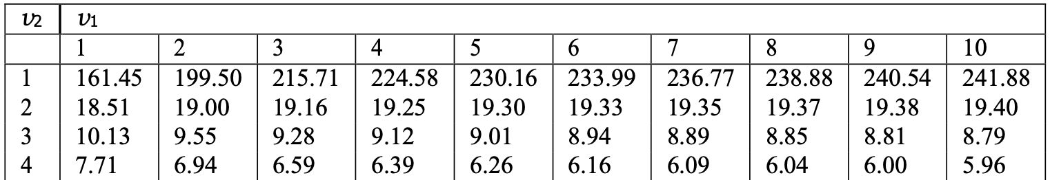
The values F_{\nu_1,\nu_2}(0.05) listed are such that P(F_{\nu_1,\nu_2} > F_{\nu_1,\nu_2}(0.05)) = 0.05
For example F_{4,3}(0.05) = 9.12

Computing F-statistic with tables

Sometimes the value F_{\nu_1,\nu_2}(0.05) is missing from F-table
In such case approximate F_{\nu_1,\nu_2}(0.05) with average of closest entries available

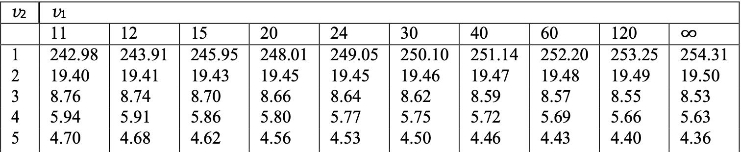
Example: F_{21,5}(0.05) is missing. We can approximate it by F_{21,5}(0.05) \approx \frac{F_{20,5}(0.05) + F_{24,5}(0.05)}{2} = \frac{ 4.56 + 4.53 }{ 2 } = 4.545

The two-sample F-test

Procedure

Suppose given two independent samples

sample x_1, \ldots, x_n from N(\mu_X,\sigma^2) of size n
sample y_1, \ldots, y_m from N(\mu_Y,\sigma^2) of size m

The one-sided hypothesis test for difference in variances is H_0 \colon \sigma^2_X = \sigma^2_Y \quad \qquad H_1 \colon \sigma^2_X > \sigma^2_Y

The two-sample F-test consists of 3 steps

The two-sample F-test

Procedure

Calculation: Compute the two-sample F-statistic F = \frac{ s_X^2}{ s_Y^2} where sample variances are s_X^2 = \frac{\sum_{i=1}^n x_i^2 - n \overline{x}^2}{n-1} \qquad \quad s_Y^2 = \frac{\sum_{i=1}^m y_i^2 - m \overline{y}^2}{m-1}

s_X^2 refers to sample with largest variance
This way s_X^2 > s_Y^2, so that F > 1

The two-sample F-test

Procedure

Statistical Tables or R: Find either
- Critical value in Tables 13.2, 13.3 F_{n-1,m-1} (0.05)
- p-value in R p := P( F_{n - 1, m-1} > |F| )

The two-sample F-test

Procedure

Interpretation:
- Reject H_0 if |F| > F_{n - 1, m-1} (0.05) \qquad \text{ or } \qquad p < 0.05
- Do not reject H_0 if |F| \leq F_{n -1, m-1} (0.05) \qquad \text{ or } \qquad p \geq 0.05

The two-sample F-test in R

Procedure using `var.test`

Store the samples x_1,\ldots,x_n and y_1,\ldots,y_m in two R vectors
- x_sample <- c(x1, ..., xn)
- y_sample <- c(y1, ..., ym)
Perform a two-sample one-sided F-test on x_sample and y_sample
- var.test(x_sample, y_sample, alternative = "greater")
Read output
- Output is similar to two-sample t-test
- The main quantity of interest is p-value

Note: alternative = "greater" specifies alternative hypothesis \sigma_X^2 > \sigma_Y^2

Part 5:
Two-sample F-test
Example

Two-sample F-test

Example

Samples: Back to example of wages of 10 Mathematicians and 13 Accountants
Assumptions: Wages are independent and normally distributed
Goal: Compare variance of wages for the 2 professions
- Is there evidence of differences in how spread out pays are?

Mathematicians	x_1	x_2	x_3	x_4	x_5	x_6	x_7	x_8	x_9	x_{10}
Wages	36	40	46	54	57	58	59	60	62	63

Accountants	y_1	y_2	y_3	y_4	y_5	y_6	y_7	y_8	y_9	y_{10}	y_{11}	y_{12}	y_{13}
Wages	37	37	42	44	46	48	54	56	59	60	60	64	64

Calculations: First sample

Repeat calculations of Slide 43

Sample size: \ n = No. of Mathematicians = 10
Mean: \bar{x} = \frac{\sum_{i=1}^n x_i}{n} = \frac{36+40+46+ \ldots +62+63}{10}=\frac{535}{10}=53.5
Variance: \begin{align*} \sum_{i=1}^n x_i^2 & = 36^2+40^2+46^2+ \ldots +62^2+63^2 = 29435 \\ s^2_X & = \frac{\sum_{i=1}^n x_i^2 - n \bar{x}^2}{n -1 } = \frac{29435-10(53.5)^2}{9} = 90.2778 \end{align*}

Calculations: Second sample

Repeat calculations of Slide 44

Sample size: \ m = No. of Accountants = 13
Mean: \bar{y} = \frac{37+37+42+ \dots +64+64}{13} = \frac{671}{13} = 51.6154
Variance: \begin{align*} \sum_{i=1}^m y_i^2 & = 37^2+37^2+42^2+ \ldots +64^2+64^2 = 35783 \\ s^2_Y & = \frac{\sum_{i=1}^m y_i^2 - m \bar{y}^2}{m - 1} = \frac{35783-13(51.6154)^2}{12} = 95.7547 \end{align*}

Calculations: F-statistic

Calculation:
- Notice that s^2_Y = 95.7547 > 90.2778 = s_X^2
- Hence the F-statistic is F = \frac{s^2_Y}{s_X^2} = \frac{95.7547}{90.2778} = 1.061\ \quad (3\ \text{d.p.})
- Note: We have swapped role of s^2_X and s^2_Y, since s^2_Y > s^2_X

Completing the F-test

Referencing Tables:
- Degrees of freedom are n - 1 = 10 - 1 = 9 \,, \qquad m - 1 = 13 - 1 = 12
- Note: Since we have swapped role of s^2_X and s^2_Y, we have F = \frac{s^2_Y}{s_X^2} \sim F_{m-1,n-1} = F_{12,9}
- Find corresponding critical value in Tables 13.2, 13.3 F_{12, 9}(0.05) = 3.07

Completing the F-test

Interpretation:
- We have that F = 1.061 < 3.07 = F_{12, 9}(0.05)
- Therefore the p-value satisfies p > 0.05
- There is no evidence (p > 0.05) in favor of H_1
- Hence we accept that \sigma_X^2 = \sigma_Y^2
Conclusion: Wage levels for the two groups appear to be equally well spread out

The F-test in R

We present two F-test solutions in R

Simple solution using the command var.test
A first-principles construction closer to our earlier hand calculation

Simple solution: Code

# Enter Wages data in 2 vectors using function c()

mathematicians <- c(36, 40, 46, 54, 57, 58, 59, 60, 62, 63)
accountants <- c(37, 37, 42, 44, 46, 48, 54, 56, 59, 60, 60, 64, 64)


# Perform one-sided F-test using var.test
# Store result of var.test in ans

ans <- var.test(accountants, mathematicians, alternative = "greater")


# Print answer
print(ans)

Note: accountants is first because it has larger variance
Code can be downloaded here F_test.R

Simple solution: Output


    F test to compare two variances

data:  accountants and mathematicians
F = 1.0607, num df = 12, denom df = 9, p-value = 0.4753
alternative hypothesis: true ratio of variances is greater than 1
95 percent confidence interval:
 0.3451691       Inf
sample estimates:
ratio of variances 
          1.060686

Comments:

First line: R tells us that an F-test is performed
Second line: Data for F-test is accountants and mathematicians

Simple solution: Output


    F test to compare two variances

data:  accountants and mathematicians
F = 1.0607, num df = 12, denom df = 9, p-value = 0.4753
alternative hypothesis: true ratio of variances is greater than 1
95 percent confidence interval:
 0.3451691       Inf
sample estimates:
ratio of variances 
          1.060686

Comments:

The F-statistic computed is F = 1.0607
- Note: This coincides with the one computed by hand (up to rounding error)

Simple solution: Output


    F test to compare two variances

data:  accountants and mathematicians
F = 1.0607, num df = 12, denom df = 9, p-value = 0.4753
alternative hypothesis: true ratio of variances is greater than 1
95 percent confidence interval:
 0.3451691       Inf
sample estimates:
ratio of variances 
          1.060686

Comments:

Numerator of F-statistic has 12 degrees of freedom
Denominator of F-statistic has 9 degrees of freedom
p-value is p = 0.4753

Simple solution: Output


    F test to compare two variances

data:  accountants and mathematicians
F = 1.0607, num df = 12, denom df = 9, p-value = 0.4753
alternative hypothesis: true ratio of variances is greater than 1
95 percent confidence interval:
 0.3451691       Inf
sample estimates:
ratio of variances 
          1.060686

Comments:

Fourth line: The alternative hypothesis is that ratio of variances is \, > 1
- This translates to H_1 \colon \sigma_X^2 > \sigma^2_Y
- Warning: This is not saying to reject H_0 – R is just stating H_1

Simple solution: Output


    F test to compare two variances

data:  accountants and mathematicians
F = 1.0607, num df = 12, denom df = 9, p-value = 0.4753
alternative hypothesis: true ratio of variances is greater than 1
95 percent confidence interval:
 0.3451691       Inf
sample estimates:
ratio of variances 
          1.060686

Comments:

Fifth line: R computes a 95 \% confidence interval for ratio \sigma_Y^2/\sigma_X^2
- Based on the data, the set of hypothetical values for \sigma_Y^2/\sigma_X^2 is (\sigma_Y^2/\sigma_X^2 ) \in [0.3451691, \infty]

Simple solution: Output


    F test to compare two variances

data:  accountants and mathematicians
F = 1.0607, num df = 12, denom df = 9, p-value = 0.4753
alternative hypothesis: true ratio of variances is greater than 1
95 percent confidence interval:
 0.3451691       Inf
sample estimates:
ratio of variances 
          1.060686

Comments:

Seventh line: R computes ratio of sample variances
- We have that s_Y^2/s_X^2 = 1.060686
- By definition the above coincides with F-statistic (up to rounding)

Simple solution: Output


    F test to compare two variances

data:  accountants and mathematicians
F = 1.0607, num df = 12, denom df = 9, p-value = 0.4753
alternative hypothesis: true ratio of variances is greater than 1
95 percent confidence interval:
 0.3451691       Inf
sample estimates:
ratio of variances 
          1.060686

Conclusion: The p-value is p = 0.4753

Since p > 0.05 we do not reject H_0
Hence \sigma^2_X and \sigma^2_Y appear to be similar
Wage levels for the two groups appear to be equally well spread out

First principles solution: Code

Start by entering data into R

# Enter Wages data in 2 vectors using function c()

mathematicians <- c(36, 40, 46, 54, 57, 58, 59, 60, 62, 63)
accountants <- c(37, 37, 42, 44, 46, 48, 54, 56, 59, 60, 60, 64, 64)

First principles solution: Code

Check which population has higher variance
In our case accountants has higher variance

# Check which variance is higher

cat("\n Variance of accountants is", var(accountants))
cat("\n Variance of mathematicians is", var(mathematicians))

First principles solution: Code

Compute sample sizes

# Calculate sample sizes

n <- length(mathematicians)
m <- length(accountants)

First principles solution: Code

Compute F-statistic F = \frac{s_Y^2}{s_X^2}
Recall: Numerator has to have larger variance
In our case accountants is numerator

# Compute F-statistics
# Numerator is population with largest variance

F <- var(accountants) / var(mathematicians)

First principles solution: Code

Compute the p-value p = P(F_{m-1, n-1} > F) = 1 - P(F_{m-1, n-1} \leq F)

# Compute p-value
p_value <- 1 - pf(F, df1 = m - 1, df2 = n - 1)

# Print p-value
cat("\n The p-value for one-sided F-test is", p_value)

Note: The command pf(f, df1 = n, df2 = m) computes probability P(F_{n,m} \leq f)

First principles solution: Output

Full code be downloaded here F_test_first_principles.R
Running the code yields the output:


 Variance of accountants is 95.75641


 Variance of mathematicians is 90.27778


 The p-value for one-sided F-test is 0.4752684

Since p > 0.05 we do not reject H_0

Statistical Models

Lecture 6: Two-samplehypothesis tests

Outline of Lecture 6

Part 1: Two-sample hypothesis tests

Overview

Problem statement

Why is this important?

Normal distribution family in action

Two-sample t-test

Normal distribution family in action

Two-sample F-test

Normal distribution family in action

Two-sample F-test

Part 2: Two-sample t-test

The two-sample t-test

The two-sample t-test

The two-sample t-statistic

The two-sample t-statistic

The two-sample t-statistic

A note on the degrees of freedom (df)

The estimated standard error

The estimated standard error

The estimated standard error

Estimating the variance

Estimating the variance

Estimating the variance

Estimating the variance

Pooled estimator of variance

The two-sample t-statistic

The two-sample t-statistic

Distribution of two-sample t-statistic

Distribution of two-sample t-statistic

Proof

Distribution of two-sample t-statistic

Proof

Distribution of two-sample t-statistic

Proof

Distribution of two-sample t-statistic

Proof

Distribution of two-sample t-statistic

Proof

Distribution of two-sample t-statistic

Proof

The two-sample t-test

Procedure

The two-sample t-test

Procedure

The two-sample t-test

Procedure

The two-sample t-test

Procedure

The two-sample t-test in R

General commands

t-test command options

Comments on command t.test(x, y)

t-test command options

Comments on command t.test(x, y)

t-test command options

Comments on command t.test(x, y)

t-test command options

Comments on command t.test(x, y)

t-test command options

Comments on command t.test(x, y)

Part 3: Two-sample t-testExample

Two-sample t-test

Example

Calculations: First sample

Calculations: Second sample

Calculations: Pooled Variance

Calculations: t-statistic

Completing the t-test

Completing the t-test

The two-sample t-test in R: Code

The two-sample t-test in R: Output

The two-sample t-test in R: Output

The two-sample t-test in R: Output

The two-sample t-test in R: Output

The two-sample t-test in R: Output

The two-sample t-test in R: Output

t-test without assuming same variance

Lecture 6:
Two-sample
hypothesis tests

Part 1:
Two-sample
hypothesis tests

Part 2:
Two-sample t-test

Comments on command `t.test(x, y)`

Comments on command `t.test(x, y)`

Comments on command `t.test(x, y)`

Comments on command `t.test(x, y)`

Comments on command `t.test(x, y)`

Part 3:
Two-sample t-test
Example

Part 4:
Two-sample F-test

Procedure using `var.test`

Part 5:
Two-sample F-test
Example