Statistical Models

Lecture 5

Dr. Silvio Fanzon

S.Fanzon@hull.ac.uk

University of Hull

Dr. John Fry

J.M.Fry@hull.ac.uk

University of Hull

Lecture 5:
Hypothesis tests in R
Part 2

Outline of Lecture 5

One-sample variance test
One-sample variance test: Example
F-distribution

Part 1:
One-sample variance test

Estimating mean and variance

Suppose to have a population with normal distribution N(\mu,\sigma^2)
- Mean \mu and variance \sigma^2 are unknown
Questions about \mu and \sigma^2
1. What is my best guess of the value?
2. How far away from the true value am I likely to be?
Answers:
- The one-sample t-test answers questions about \mu
- The one-sample variance ratio test answers questions about \sigma^2

Chi-squared distribution

The-one sample variance test uses chi-squared distribution
Recall: Chi-squared distribution with p degrees of freedom is \chi_p^2 = Z_1^2 + \ldots + Z_p^2 where Z_1, \ldots, Z_p are iid N(0, 1)

One-sample one-sided variance ratio test

Assumption: Suppose given sample X_1,\ldots, X_n iid from N(\mu,\sigma^2)

Goal: Estimate variance \sigma^2 of population

Test:

Suppose \sigma_0 is guess for \sigma
The one-sided hypothesis test for \sigma is H_0 \colon \sigma = \sigma_0 \qquad H_1 \colon \sigma > \sigma_0

One-sample one-sided variance ratio test

What to do?

Consider the sample variance S^2 = \frac{ \sum_{i=1}^n X_i^2 - n \overline{X}^2 }{n-1}
Since we believe H_0, the variance is \sigma = \sigma_0
S^2 cannot be too far from the true variance \sigma
Therefore we cannot have that S^2 \gg \sigma^2 = \sigma_0^2

One-sample one-sided variance ratio test

What to do?

If we observe S^2 \gg \sigma_0^2 then our guess \sigma_0 is probably wrong
Therefore we reject H_0 if S^2 \gg \sigma_0^2
The rejection condition S^2 \gg \sigma_0^2 is equivalent to \frac{(n-1)S^2}{\sigma_0^2} \gg 1 where n is the sample size

One-sample one-sided variance ratio test

What to do?

We define our test statistic as \chi^2 := \frac{(n-1)s^2}{\sigma_0^2}
The rejection condition is hence \chi^2 \gg 1

One-sample one-sided variance ratio test

What to do?

Recall that \frac{(n-1)S^2}{\sigma^2} \sim \chi_{n-1}^2
Assuming \sigma=\sigma_0, we therefore have \chi^2 = \frac{(n-1)S^2}{\sigma_0^2} = \frac{(n-1)S^2}{\sigma^2} \sim \chi_{n-1}^2

One-sample one-sided variance ratio test

Summary

We reject H_0 if \chi^2 = \frac{(n-1)S^2}{\sigma_0^2} \gg 1
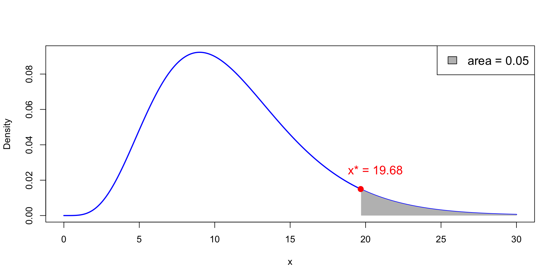
As \chi^2 \sim \chi_{n-1}^2, we decide to rejct H_0 if \chi^2 > \chi_{n-1}^2(0.05)
By definition the critical value \chi_{n-1}^2(0.05) is such that P(\chi_{n-1}^2 > \chi_{n-1}^2(0.05) ) = 0.05

Critical values of chi-squared

x^* := \chi_{n-1}^2(0.05) is point on x-axis such that P(\chi_{n-1}^2 > x^* ) = 0.05
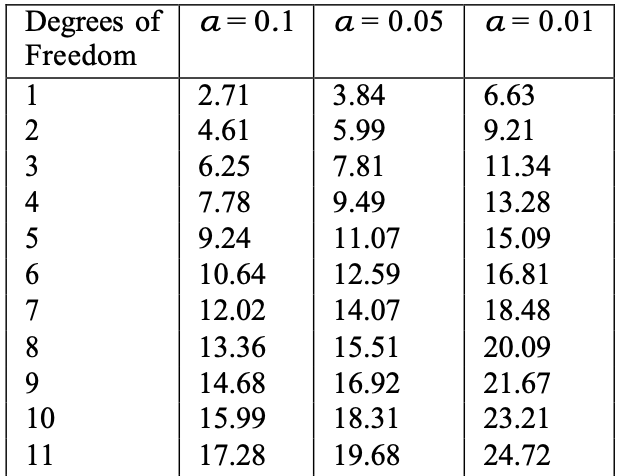
In the picture we have n = 12 and \chi_{11}^2(0.05) = 19.68

Critical values of chi-squared – Tables

Find Table 13.5 in this file
Look at the row with Degree of Freedom n-1 (or its closest value)
Find critical value \chi^2_{n-1}(0.05) in column \alpha = 0.05
Example: n=12, DF =11, \chi^2_{11}(0.05) = 19.68

One-sample one-sided variance ratio test

p-value

Given the test statistic \chi^2 the p-value is defined as p := P( \chi_{n-1}^2 > \chi^2 )
Notice that p < 0.05 \qquad \iff \qquad \chi^2 > \chi_{n-1}^2(0.05)

This is because \chi^2 > \chi_{n-1}^2(0.05) iff p = P(\chi_{n-1}^2 > \chi^2) < P(\chi_{n-1}^2 > \chi_{n-1}^2(0.05) ) = 0.05

One-sample one-sided variance ratio test

Procedure

Suppose given

Sample x_1, \ldots, x_n of size n from N(\mu,\sigma^2)
Guess \sigma_0 for \sigma

The one-sided hypothesis test is H_0 \colon \sigma = \sigma_0 \qquad H_1 \colon \sigma > \sigma_0 The variance ratio test consists of 3 steps

One-sample one-sided variance ratio test

Procedure

Calculation: Compute the chi-squared statistic \chi^2 = \frac{(n-1) s^2}{\sigma_0^2} where sample mean and variance are \overline{x} = \frac{1}{n} \sum_{i=1}^n x_i \,, \qquad s^2 = \frac{\sum_{i=1}^n x_i^2 - n \overline{x}^2}{n-1}

One-sample one-sided variance ratio test

Procedure

Statistical Tables or R: Find either
- Critical value in Table 13.5 \chi_{n-1}^2(0.05)
- p-value in R p := P( \chi_{n-1}^2 > \chi^2 )

One-sample one-sided variance ratio test

Procedure

Interpretation:
- Reject H_0 if \chi^2 > \chi_{n-1}^2(0.05) \qquad \text{ or } \qquad p < 0.05
- Do not reject H_0 if \chi^2 \leq \chi_{n-1}^2(0.05) \qquad \text{ or } \qquad p \geq 0.05

Part 2:
One-sample variance test: Example

One-sample variance ratio test: Example

Month	J	F	M	A	M	J	J	A	S	O	N	D
Cons. Expectation	66	53	62	61	78	72	65	64	61	50	55	51
Cons. Spending	72	55	69	65	82	77	72	78	77	75	77	77
Difference	-6	-2	-7	-4	-4	-5	-7	-14	-16	-25	-22	-26

Data: Consumer Expectation (CE) and Consumer Spending (CS) in 2011
Assumption: CE and CS are normally distributed

One-sample variance ratio test: Example

Month	J	F	M	A	M	J	J	A	S	O	N	D
Cons. Expectation	66	53	62	61	78	72	65	64	61	50	55	51
Cons. Spending	72	55	69	65	82	77	72	78	77	75	77	77
Difference	-6	-2	-7	-4	-4	-5	-7	-14	-16	-25	-22	-26

Remark: Monthly data on CE and CS can be matched
- Hence consider: \quad Difference = CE - CS
- CE and CS normal \quad \implies \quad Difference \sim N(\mu,\sigma^2)
Question: Test the following hypothesis: H_0 \colon \sigma = 1 \qquad H_1 \colon \sigma > 1

Motivation of test

If X \sim N(\mu,\sigma^2) then P( \mu - 2 \sigma \leq X \leq \mu + 2\sigma ) \approx 0.95
Recall: \quad Difference = (CE - CS) \sim N(\mu,\sigma^2)
Hence if \sigma = 1 P( \mu - 2 \leq {\rm CE} - {\rm CS} \leq \mu + 2 ) \approx 0.95
Meaning of variance ratio test: \sigma=1 \quad \implies \quad \text{CS index is within } \pm{2\sigma} \text{ of CE index with probability } 0.95

The variance ratio test

Month	J	F	M	A	M	J	J	A	S	O	N	D
Difference	-6	-2	-7	-4	-4	-5	-7	-14	-16	-25	-22	-26

Calculations: With data on Difference compute

Sample mean: \bar{x} = \frac{\sum_{i=1}^{n} x_i}{n} = \frac{-6-2-7-4- \ldots -22-26}{12} = -\frac{138}{12} = -11.5

The variance ratio test

Month	J	F	M	A	M	J	J	A	S	O	N	D
Difference	-6	-2	-7	-4	-4	-5	-7	-14	-16	-25	-22	-26

Calculations: With data on Difference compute

Sample variance: \begin{align*} \sum_{i=1}^{n} x_i^2 & = (-6)^2 + (-2)^2 + (-7)^2 + \ldots + (-22)^2 + (-26)^2 = 2432 \\ s^2 & = \frac{\sum_{i=1}^n x^2_i- n \bar{x}^2}{n-1} = \frac{2432-12(-11.5)^2}{11} = \frac{845}{11} = 76.8182 \end{align*}

The variance ratio test

Month	J	F	M	A	M	J	J	A	S	O	N	D
Difference	-6	-2	-7	-4	-4	-5	-7	-14	-16	-25	-22	-26

Calculations: With data on Difference compute

Chi-squared statistic: \chi^2 = \frac{(n-1)s^2}{\sigma_0^2} = \frac{11 \left(\frac{845}{11}\right) }{1} = 845

The variance ratio test

Statistical Tables:
- Sample size is n = 12
- In Table 13.5 find \chi_{11}^2(0.05) = 19.68
Interpretation:
- Test statistic is \chi^2 = 845
- We reject H_0 because \chi^2 = 845 > 19.68 = \chi_{n-1}^2(0.05)

The variance ratio test

Conclusion:
- We accept H_1: The standard deviation satisfies \sigma > 1
- A better estimate for \sigma could be sample standard deviation s=\sqrt{\frac{845}{11}}=8.765
- This suggests: With probability 0.95 \text{CS index is within } \pm{2 \times 8.765 = \pm 17.53 } \text{ of CE index}

The variance ratio test in R

Goal: Perform chi-squared variance ratio test in R

For this we need to compute p-value p = P(\chi_{n-1}^2 > \chi^2)
Thus, we need to compute probabilities for chi-squared distribution in R

Probability Distributions in R

R can natively do calculations with known probability distrubutions
Example: Let X be r.v. with N(\mu,\sigma^2) distribution

R command	Meaning
`pnorm(x, mean = mu, sd = sig)`	P(X \leq x)
`qnorm(p, mean = mu, sd = sig)`	P(X \leq q) = p
`dnorm(x, mean = mu, sd = sig)`	f(x) where f is distr. of X
`rnorm(n, mean = mu, sd = sig)`	n random samples from distr. of X

Note: Syntax of commands

norm = normal \qquad p = probability \qquad q = quantile

d = distribution \qquad r = random

Probability Distributions in R

Example

Suppose average height of women is normally distributed N(\mu,\sigma^2)
Assume mean \mu = 163 cm and standard deviation \sigma = 8 cm

# Probability woman exceeds 180cm in height
# P(X > 180) = 1 - P(X <= 180)

1 - pnorm(180, mean = 163, sd = 8)

[1] 0.01679331

Probability Distributions in R

Example

Suppose average height of women is normally distributed N(\mu,\sigma^2)
Assume mean \mu = 163 cm and standard deviation \sigma = 8 cm

# The upper 10th percentile for women height, that is,
# height q such that P(X <= q) = 0.9

qnorm(0.90, mean = 163, sd = 8)

[1] 173.2524

Probability Distributions in R

Example

Suppose average height of women is normally distributed N(\mu,\sigma^2)
Assume mean \mu = 163 cm and standard deviation \sigma = 8 cm

# Value of density at 163

dnorm(163, mean = 163, sd = 8)

[1] 0.04986779

Probability Distributions in R

Example

Suppose average height of women is normally distributed N(\mu,\sigma^2)
Assume mean \mu = 163 cm and standard deviation \sigma = 8 cm

# Generate random sample of size 5

rnorm(5, mean = 163, sd = 8)

[1] 166.5672 160.5149 153.1829 161.2974 161.9265

Probability Distributions in R

Chi-squared distribution

Commands for chi-squared distrubution are similar
df = n denotes n degrees of feedom

R command	Meaning
`pchisq(x, df = n)`	P(X \leq x)
`qchisq(p, df = n)`	P(X \leq q) = p
`dchisq(x, df = n)`	f(x) where f is distr. of X
`rchisq(m, df = n)`	m random samples from distr. of X

Probability Distributions in R

Example 1

From Tables we found quantile \chi_{11}^2 (0.05) = 19.68
Question: Compute such quantile in R

Probability Distributions in R

Example 1 – Solution

From Tables we found quantile \chi_{11}^2 (0.05) = 19.68
Question: Compute such quantile in R

# Compute 0.95 quantile for chi-squared with 11 degrees of freedom

quantile <- qchisq(0.95, df = 11)

cat("The 0.95 quantile for chi-squared with df = 11 is", quantile)

The 0.95 quantile for chi-squared with df = 11 is 19.67514

Probability Distributions in R

Example 2

The \chi^2 statistic for variance ratio test has distribution \chi_{n-1}^2
Question: Compute the p-value p := P(\chi_{n-1}^2 > \chi^2)

Probability Distributions in R

Example 2 – Solution

The \chi^2 statistic for variance ratio test has distribution \chi_{n-1}^2
Question: Compute the p-value p := P(\chi_{n-1}^2 > \chi^2)
Observe that p := P(\chi_{n-1}^2 > \chi^2) = 1 - P(\chi_{n-1}^2 \leq \chi^2)
The code is therefore

# Compute p-value for chi^2 = chi_squared and df = n

p_value <- 1 - pchisq(chi_squared, df = n)

The variance ratio test in R

Month	J	F	M	A	M	J	J	A	S	O	N	D
Cons. Expectation	66	53	62	61	78	72	65	64	61	50	55	51
Cons. Spending	72	55	69	65	82	77	72	78	77	75	77	77
Difference	-6	-2	-7	-4	-4	-5	-7	-14	-16	-25	-22	-26

Back to Example: Monthly data on CE and CS
Question: Test the following hypothesis: H_0 \colon \sigma = 1 \qquad H_1 \colon \sigma > 1

The variance ratio test in R

Month	J	F	M	A	M	J	J	A	S	O	N	D
Cons. Expectation	66	53	62	61	78	72	65	64	61	50	55	51
Cons. Spending	72	55	69	65	82	77	72	78	77	75	77	77
Difference	-6	-2	-7	-4	-4	-5	-7	-14	-16	-25	-22	-26

Start by entering data into R

# Enter Consumer Expectation and Consumer Spending data
CE <- c(66, 53, 62, 61, 78, 72, 65, 64, 61, 50, 55, 51)
CS <- c(72, 55, 69, 65, 82, 77, 72, 78, 77, 75, 77, 77)

# Compute difference
difference <- CE - CS

The variance ratio test in R

Compute chi-squared statistic \chi^2 = \frac{(n-1) s^2}{\sigma^2_0}

# Compute sample size
n <- length(difference)

# Enter null hypothesis
sigma_0 <- 1

# Compute sample variance
variance <- var(difference)

# Compute chi-squared statistic
chi_squared <- (n - 1) * variance / sigma_0 ^ 2

The variance ratio test in R

Compute the p-value p = P(\chi_{n-1}^2 > \chi^2) = 1 - P(\chi_{n-1}^2 \leq \chi^2)

# Compute p-value
p_value <- 1 - pchisq(chi_squared, df = n - 1)

# Print p-value
cat("The p-value for one-sided variance test is", p_value)

The full code can be downloaded here variance_ratio_test.R

Running the code

Running variance_ratio_test.R gives the following output:

The p-value for one-sided variance test is 0

Since p < 0.05 we reject H_0
Therefore the true variance seems to be \sigma^2 > 1

Part 3:
F-distribution

Overview

Chi-squared distribution

Recall: Chi-squared distribution with p degrees of freedom is \chi_p^2 = Z_1^2 + \ldots + Z_p^2 where Z_1, \ldots, Z_n are iid N(0, 1)

Overview

Chi-squared distribution

Chi-squared distribution was used to:

Describe distribution of sample variance S^2: \frac{(n-1)S^2}{\sigma^2} \sim \chi_{n-1}^2
Define t-distribution: t_p \sim \frac{U}{\sqrt{V/p}} where U \sim N(0,1) and V \sim \chi_p^2

F-distribution

F-distribution is:

Defined in terms of ratio of \chi_p^2
Describes variance estimators for independent samples

F-distribution

Definition

The r.v. F has F-distribution with p and q degrees of freedom if the pdf is f_F(x) = \frac{ \Gamma \left(\frac{p+q}{2} \right) }{ \Gamma \left( \frac{p}{2} \right) \Gamma \left( \frac{q}{2} \right) } \left( \frac{p}{q} \right)^{p/2} \, \frac{ x^{ (p/2) - 1 } }{ [ 1 + (p/q) x ]^{(p+q)/2} } \,, \quad x > 0

Notation: F-distribution with p and q degrees of freedom is denoted by F_{p,q}

F-distribution

The F-distribution is obtained as ratio of 2 independent chi-squared distributions

Theorem

Suppose that U \sim \chi_p^2 and V \sim \chi_q^2 are independent. Then X := \frac{U/p}{V/q} \sim F_{p,q}

F-distribution

Idea of Proof

Similar to the proof (seen in Homework 3) that \frac{U}{\sqrt{V/p}} \sim t_p where U \sim N(0,1) and V \sim \chi_p^2 are independent
In our case we need to prove X := \frac{U/p}{V/q} \sim F_{p,q} where U \sim \chi_p^2 and V \sim \chi_q^2 are independent

F-distribution

Idea of Proof

U \sim \chi_{p}^2 and V \sim \chi_q^2 are independent. Therefore \begin{align*} f_{U,V} (u,v) & = f_U(u) f_V(v) \\ & = \frac{ 1 }{ \Gamma \left( \frac{p}{2} \right) \Gamma \left( \frac{q}{2} \right) 2^{(p+q)/2} } u^{\frac{p}{2} - 1} v^{\frac{q}{2} - 1} e^{-(u+v)/2} \end{align*}
Consider the change of variables x(u,v) := \frac{u/p}{v/q} \,, \quad y(u,v) := u + v

F-distribution

Idea of Proof

This way we have X = \frac{U/p}{V/q} \,, \qquad Y = U + V
We can compute f_X via f_{X}(x) = \int_{0}^\infty f_{X,Y}(x,y) \, dy

F-distribution

Idea of Proof

The joint pdf f_{X,Y} can be computed by inverting the change of variables x(u,v) := \frac{u/p}{v/q} \,, \quad y(u,v) := u + v and using the formula f_{X,Y}(x,y) = f_{U,V}(u(x,y),v(x,y)) \, |\det J| where J is the Jacobian of the inverse transformation (x,y) \mapsto (u(x,y),v(x,y))

F-distribution

Idea of Proof

Since f_{U,V} is known, then also f_{X,Y} is known
Moreover the integral f_{X}(x) = \int_{0}^\infty f_{X,Y}(x,y) \, dy can be explicitly computed, yielding the thesis f_{X}(x) = \frac{ \Gamma \left(\frac{p+q}{2} \right) }{ \Gamma \left( \frac{p}{2} \right) \Gamma \left( \frac{q}{2} \right) } \left( \frac{p}{q} \right)^{p/2} \, \frac{ x^{ (p/2) - 1 } }{ [ 1 + (p/q) x ]^{(p+q)/2} }

Properties of F-distribution

Theorem

Suppose X \sim F_{p,q} with q>2. Then {\rm I\kern-.3em E}[X] = \frac{q}{q-2}
If X \sim F_{p,q} then 1/X \sim F_{q,p}
If X \sim t_q then X^2 \sim F_{1,q}

Properties of F-distribution

Proof of Theorem

Requires a bit of work. It will be left as Homework assignment
By the Theorem in Slide 43 we have X \sim F_{p,q} \quad \implies \quad X = \frac{U/p}{V/q} with U \sim \chi_p^2 and V \sim \chi_q^2 independent. Therefore \frac{1}{X} = \frac{V/q}{U/p} \sim F_{q,p}

Properties of F-distribution

Proof of Theorem

Suppose X \sim t_q. The Theorem in Slide 66 of Lecture 3 guarantees that X = \frac{U}{\sqrt{V/q}} where U \sim N(0,1) and V \sim \chi_q^2 are independent. Therefore X^2 = \frac{U^2}{V/q}

Properties of F-distribution

Proof of Theorem

Since U \sim N(0,1), by definition U^2 \sim \chi_1^2.
Moreover U^2 and V are independet, since U and V are independent
Theorem in Slide 43 implies X^2 = \frac{U^2}{V/q} \sim \frac{\chi_1^2/1}{\chi_q^2/q} \sim F_{1,q}

Statistical Models

Lecture 5: Hypothesis tests in R Part 2

Outline of Lecture 5

Part 1: One-sample variance test

Estimating mean and variance

Chi-squared distribution

One-sample one-sided variance ratio test

One-sample one-sided variance ratio test

What to do?

One-sample one-sided variance ratio test

What to do?

One-sample one-sided variance ratio test

What to do?

One-sample one-sided variance ratio test

What to do?

One-sample one-sided variance ratio test

Summary

Critical values of chi-squared

Critical values of chi-squared – Tables

One-sample one-sided variance ratio test

p-value

One-sample one-sided variance ratio test

Procedure

One-sample one-sided variance ratio test

Procedure

One-sample one-sided variance ratio test

Procedure

One-sample one-sided variance ratio test

Procedure

Part 2: One-sample variance test: Example

One-sample variance ratio test: Example

One-sample variance ratio test: Example

Motivation of test

The variance ratio test

The variance ratio test

The variance ratio test

The variance ratio test

The variance ratio test

The variance ratio test in R

Probability Distributions in R

Probability Distributions in R

Example

Probability Distributions in R

Example

Probability Distributions in R

Example

Probability Distributions in R

Example

Probability Distributions in R

Chi-squared distribution

Probability Distributions in R

Example 1

Probability Distributions in R

Example 1 – Solution

Probability Distributions in R

Example 2

Probability Distributions in R

Example 2 – Solution

The variance ratio test in R

The variance ratio test in R

The variance ratio test in R

The variance ratio test in R

Running the code

Part 3: F-distribution

Overview

Chi-squared distribution

Overview

Chi-squared distribution

F-distribution

F-distribution

F-distribution

F-distribution

Idea of Proof

F-distribution

Idea of Proof

F-distribution

Idea of Proof

F-distribution

Idea of Proof

F-distribution

Lecture 5:
Hypothesis tests in R
Part 2

Part 1:
One-sample variance test

Part 2:
One-sample variance test: Example

Part 3:
F-distribution