plot(rnorm(1000))Statistical Models
Lecture 4
Lecture 4:
Hypothesis tests in R
Part 1
Outline of Lecture 4
- t-test
- The basics of R
- Vectors
- t-test in R
- Graphics
Part 1:
t-test
One-sample Two-sided t-test
Goal: estimate the mean \mu of a normal population N(\mu,\sigma^2). If \mu_0 is guess for \mu H_0 \colon \mu = \mu_0 \qquad H_1 \colon \mu \neq \mu_0
- One-sample means we sample only from one population
- The variance \sigma is unknown
- Suppose the sample size is n, with sample X_1 ,\ldots,X_n
- We consider the t-statistics T = \frac{\overline{X}-\mu_0}{S/\sqrt{n}}
- Recall: T \sim t_{n-1} Student’s t-distribution with n-1 degrees of freedom
One-sample Two-sided t-test
Procedure for all tests
- Calculation
- Reference statistical tables or numerical values
- Interpretation
One-sample Two-sided t-test
Calculation
- We have n samples available x_1,\ldots,x_n
- Compute sample mean \overline{x} = \frac{1}{n} \sum_{i=1}^n x_i
- Compute the sample standard deviation s = \sqrt{\frac{\sum_{i=1}^n x_i^2 - n \overline{x}^2}{n-1}}
One-sample Two-sided t-test
Calculation
Compute the estimated standard error \mathop{\mathrm{e.s.e.}}= \frac{s}{\sqrt{n}}
Compute the t-statistic t = \frac{\text{estimate } - \text{ hypothesised value}}{\mathop{\mathrm{e.s.e.}}} = \frac{\overline x - \mu_0}{s/\sqrt{n}}
\mu_0 is the value of the null hypothesis H_0
One-sample Two-sided t-test
p-value
After computing t-statistic we need to compute p-value
p-value is a measure of how strange the data is in relation to the null hypothesis
We have 2 options:
- LOW p-value \quad \implies \quad reject H_0
- HIGH p-value \quad \implies \quad do not reject H_0
In this course we reject H_0 for p-values p<0.05
One-sample Two-sided t-test
p-value
For two-sided t-test the p-value is defined as p := 2P(t_{n-1}> |t|) where t_{n-1} is the t-distribution with n-1 degrees of freedom
Therefore the p-value is p = 2P(\text{Observing t }| \, \mu=\mu_0)
One-sample Two-sided t-test
p-value
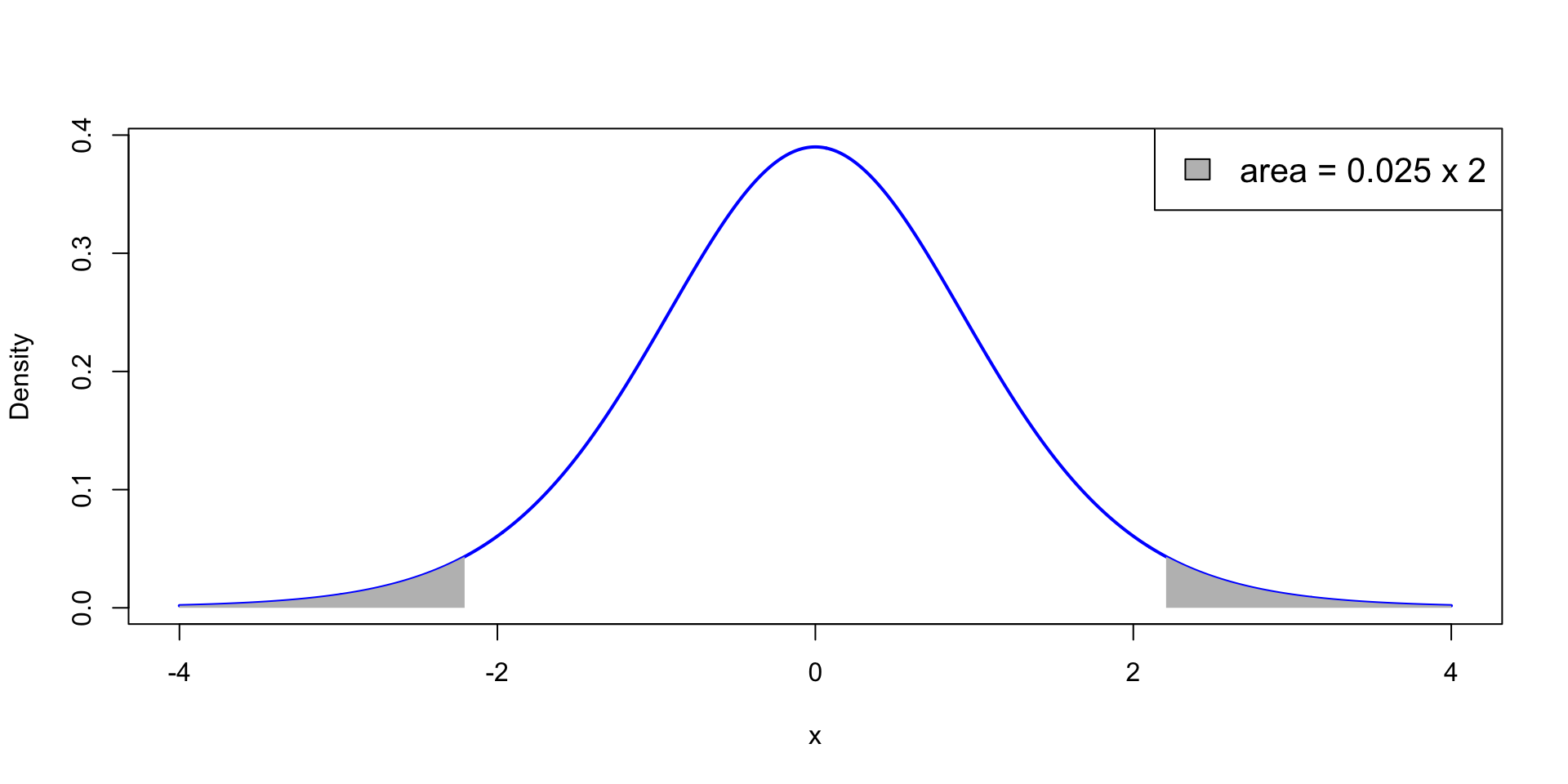
p<0.05 means that the test statistic t is extreme: \,\, P(t_{n-1}> |t|)<0.025
t falls in the grey areas in the t_{n-1} plot below: Each grey area measures 0.025
One-sample Two-sided t-test
p-value
- How to compute p?
- Use statistical tables – Available here
- Use R – Next sections
One-sample Two-sided t-test
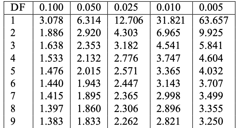
Reference statistical tables
Find Table 13.1 in this file
- Look at the row with Degree of Freedom n-1 (or its closest value)
- Find critical value t^* := t_{n-1}(0.025) in column 0.025
- Example: n=10, DF =9, t^*=t_{9}(0.025)=2.262
One-sample Two-sided t-test
Reference statistical tables
The critical value t^* = t_{n-1}(0.025) found in the table satisfies P(t_{n-1}>t^*) = 0.025
By definition of p-value for two-sided t-test we have p := 2P(t_{n-1}>|t|)
Therefore, for |t|>t^* \begin{align*} p & := 2P(t_{n-1}>|t|) \\ & < 2P(t_{n-1}>t^*) = 2 \cdot (0.025) = 0.05 \end{align*}
Conclusion: \qquad |t|>t^* \quad \iff \quad p<0.05
One-sample Two-sided t-test
Interpretation
Recall that p = 2P ( \text{Observing t } | \mu = \mu_0). We have two possibilities:
- |t|>t^*
- In this case p<0.05
- The observed statistic t is very unlikely under H_0
- We reject H_0
- |t| \leq t^*
- In this case p>0.05
- The observed statistic t is not unlikely under H_0
- We do not reject H_0
Example: 2008 crisis
- Data: Monthly Consumer Confidence Index (CCI) in 2007 and 2009
- Question: Did the crash of 2008 have lasting impact upon CCI?
- Observation: Data shows a massive drop in CCI between 2009 and 2007
- Method: Use t-test to see if data is sufficient to prove that CCI actually dropped
| Month | J | F | M | A | M | J | J | A | S | O | N | D |
|---|---|---|---|---|---|---|---|---|---|---|---|---|
| CCI 2007 | 86 | 86 | 88 | 90 | 99 | 97 | 97 | 96 | 99 | 97 | 90 | 90 |
| CCI 2009 | 24 | 22 | 21 | 21 | 19 | 18 | 17 | 18 | 21 | 23 | 22 | 21 |
| Difference | 62 | 64 | 67 | 69 | 80 | 79 | 80 | 78 | 78 | 74 | 68 | 69 |
Example: 2008 crisis
- This is really a two-sample problem – CCI data in 2 populations: 2007 and 2009
- It reduces to a one-sample problem because we have directly comparable units
- If units cannot be compared, then we must use a two-sample approach
- Two-sample approach will be discussed later
| Month | J | F | M | A | M | J | J | A | S | O | N | D |
|---|---|---|---|---|---|---|---|---|---|---|---|---|
| CCI 2007 | 86 | 86 | 88 | 90 | 99 | 97 | 97 | 96 | 99 | 97 | 90 | 90 |
| CCI 2009 | 24 | 22 | 21 | 21 | 19 | 18 | 17 | 18 | 21 | 23 | 22 | 21 |
| Difference | 62 | 64 | 67 | 69 | 80 | 79 | 80 | 78 | 78 | 74 | 68 | 69 |
Example: 2008 crisis
Setting up the test
- We want to test if there was a change in CCI from 2007 to 2009
- We are really only interested in the difference in CCI
- Let \mu be the (unknown) average difference in CCI
- The null hypothesis is that there was (on average) no change in CCI H_0 \colon \mu = 0
- The alternative hypothesis is that there was some change: H_1 \colon \mu \neq 0
- Note that this is a two-sided test
Example: 2008 crisis
Calculation
Using the available data, we need to compute:
Sample mean and standard deviation \overline{x} = \frac{1}{n} \sum_{i=1}^n x_i \qquad s = \sqrt{\frac{\sum_{i=1}^n x_i^2 - n \overline{x}^2}{n-1}}
Test statistic t = \frac{\overline x - \mu_0}{s/\sqrt{n}}
Example: 2008 crisis
Calculation
| CCI | J | F | M | A | M | J | J | A | S | O | N | D |
|---|---|---|---|---|---|---|---|---|---|---|---|---|
| Difference | 62 | 64 | 67 | 69 | 80 | 79 | 80 | 78 | 78 | 74 | 68 | 69 |
\begin{align*} \overline{x} & =\frac{1}{n} \sum_{i=1}^{n} x_i=\frac{1}{12} \left(62+64+67+{\ldots}+68+69\right)=\frac{868}{12}=72.33 \\ \sum_{i=1}^{n} x_i^2 & = 62^2+64^2+67^2+{\ldots}+68^2+69^2 = 63260 \\ s & = \sqrt{ \frac{\sum_{i=1}^n x_i^2 - n \overline{x}^2}{n-1} } = \sqrt{\frac{63260-12\left(\frac{868}{12}\right)^2}{11}} = \sqrt{\frac{474.666}{11}} = 6.5689 \end{align*}
Example: 2008 crisis
Calculation
- The sample size is n=12
- The sample mean is \overline{x}=72.33
- The sample standard deviation is s = 6.5689
- The hypothesized mean is \mu_0 = 0
- The t-statistic is t = \frac{\overline{x} - \mu_0}{s/\sqrt{n}} = \frac{72.33 - 0}{6.5689/\sqrt{12}} = 38.145
Example: 2008 crisis
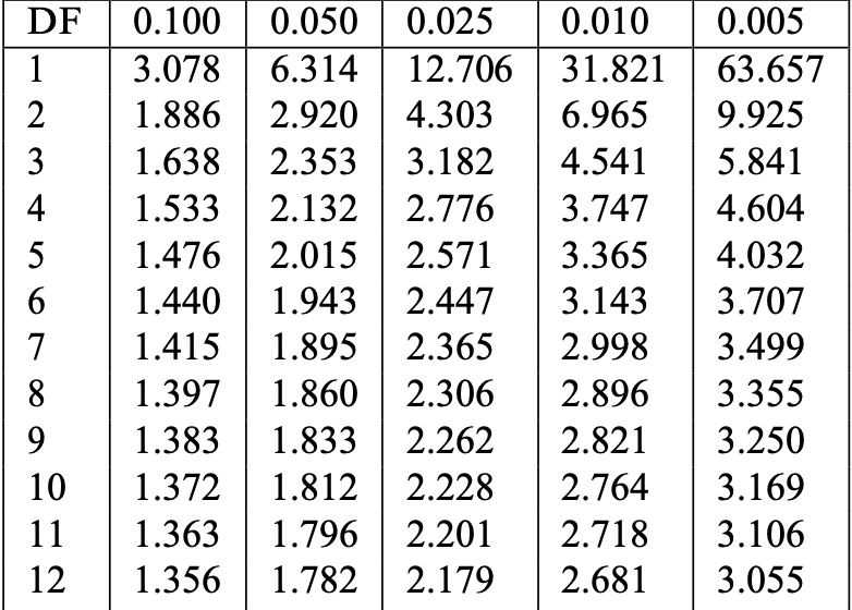
Reference statistical tables
Find Table 13.1 in this file
- Find row with DF = n-1 (or closest). Find critical value t^* in column 0.025
- In our case: n=12, DF =11, t^*= t_{11}(0.025) =2.201
Example: 2008 crisis
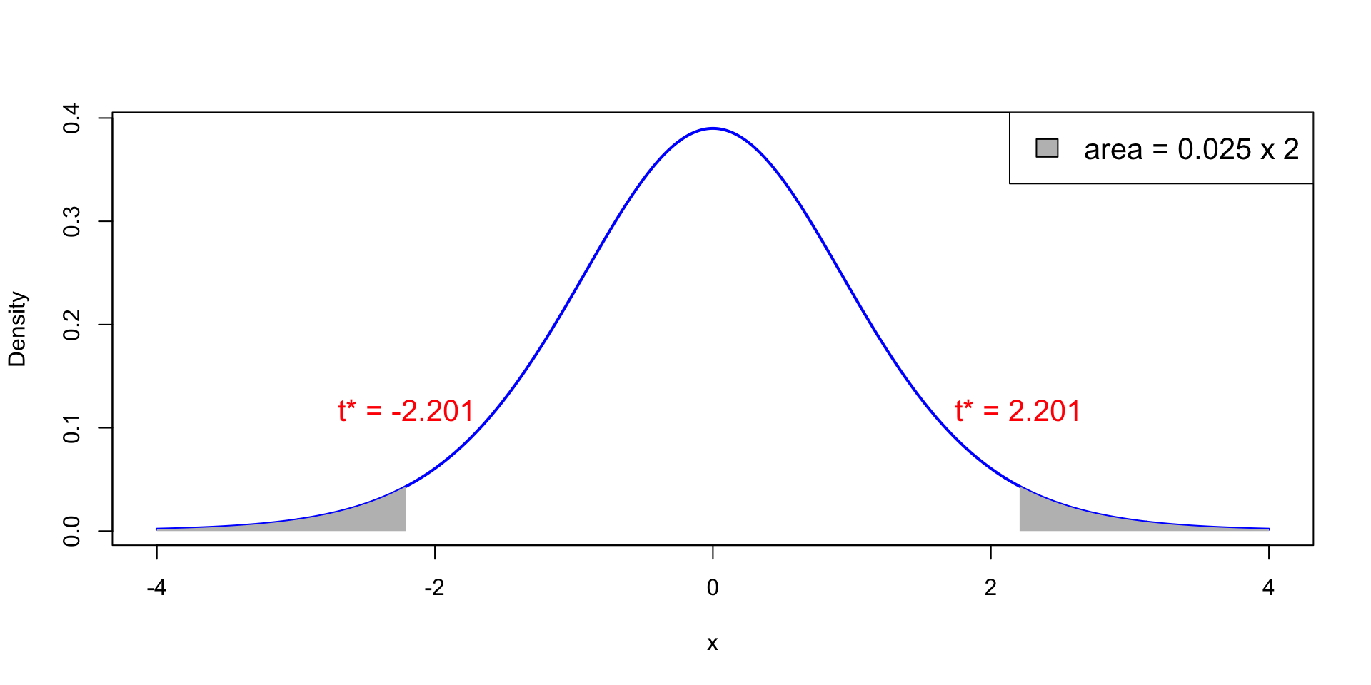
Reference statistical tables
- Plot of t_{11} distribution. White area is 0.95, total shaded area is 0.05
- Probability of observing |t|>t^* = 2.201 is p with p<0.025
Example: 2008 crisis
Interpretation
We have computed:
- Test statistic t = 38.145
- Critical value t^* = 2.201
Therefore |t| = 38.145 > 2.201 = t^*
This implies rejecting the null hypothesis H_0 \colon \mu = 0
Example: 2008 crisis
Interpretation
t-test implies that mean difference in CCI is \mu \neq 0
The sample mean difference is positive (\bar{x}=72.33)
Conclusions:
- CCI has changed from 2007 to 2009 (backed by t-test)
- CCI seems higher in 2007 than in 2009 (backed by sample mean)
- The 2008 crash seems to have reduced consumer confidence
Part 2:
The basics of R
What is R?
- R is a high-level programming language (like Python)
- This means R deals automatically with some details of computer execution:
- Memory allocation
- Resources allocation
- R is focused on manipulating and analyzing data
References
Slides are based on
Concise Statistics with R
Comprehensive R manual
Installing R
- R is freely available on Windows, Mac OS and Linux
- To install:
- Download R from CRAN https://cran.r-project.org
- Make sure you choose the right version for your system
- Follow the instructions to install
How to use R?
We have installed R. What now?
Launch the R Console. There are two ways:
- Find the R application on your machine
- Open a terminal, type R, exectute
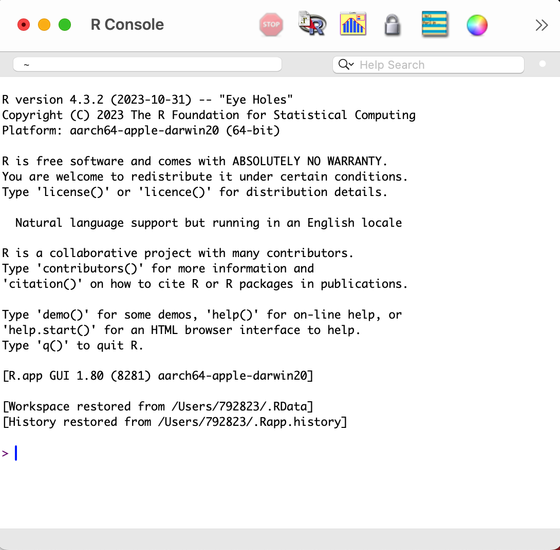
R application
This is how the R Console looks on the Mac OS app
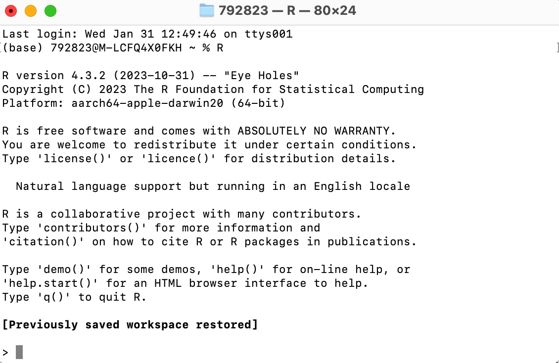
R from terminal
This is how the R Console looks on the Mac Terminal
What can R do?
- R Console is waiting for commands
- You can use the R Console interactively:
- Type a command after the symbol
> - Press
Enterto execute - R will respond
- Type a command after the symbol
Warning
- The following slides might look like a lot of information
- However you do not have to remember all the material
- It is enough to:
- Try to understand the examples
- Know that certain commands exist and what they do
- Combining commands to create complex codes comes with experience
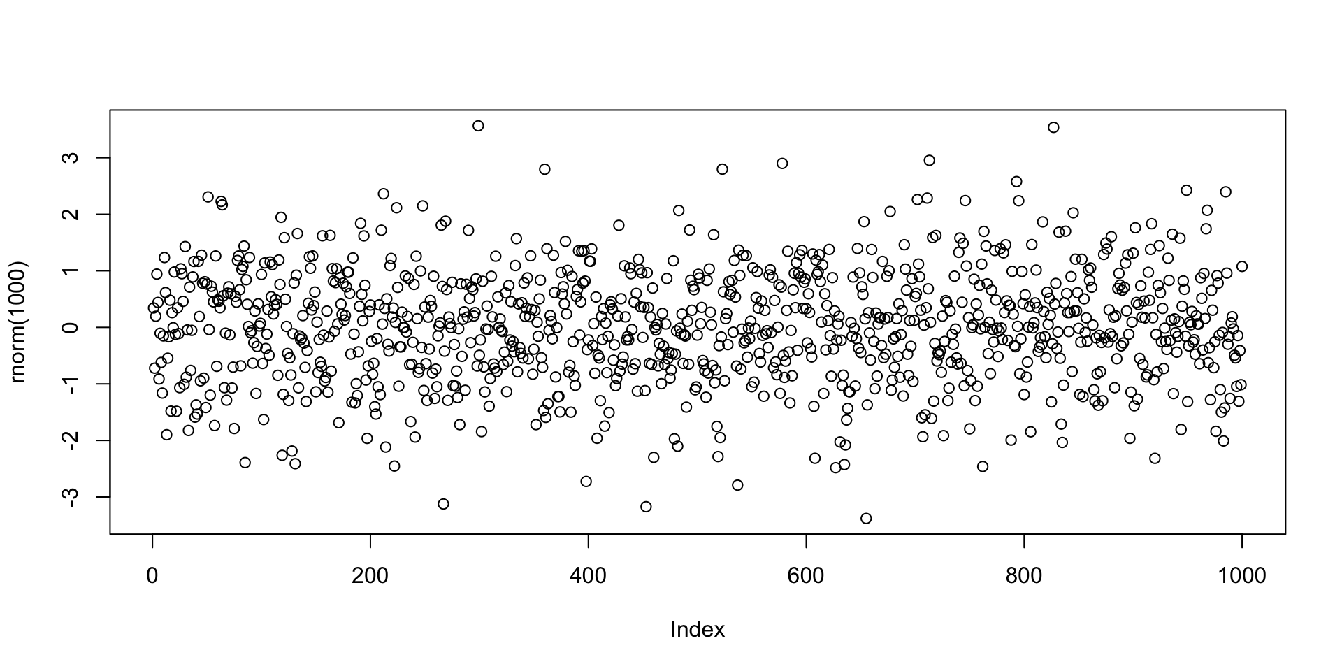
Example
Few lines of code can lead to impressive results
Example: Plotting 1000 values randomly generated from normal distribution
R as a calculator
R can perform basic mathematical operations
Below you can see R code and the corresponding answer
R Scripts
The interactive R Console is OK for short codes
For longer code use R scripts
- Write your code in a text editor
- Save your code to a plain text file with
.txtor.Rextension - Execute your code in the R Console with
source("file_name.R")
Examples of text editors
- TextPad (Windows)
- TextEdit (MacOS)
- VisualStudio Code (Cross platform)
RStudio
- RStudio is an alternative to R Console and text editors: Download here
- RStudio is an Integrated Development Environment (IDE)
- It is the R version of Spyder for Python
- RStudio includes:
- Direct-submission code editor
- Separate point-and-click panes for files, objects, and project management
- Creation of markup documents incorporating R code
Working Directory
R session has a working directory associated with it
Unless specified, R will use a default working directory
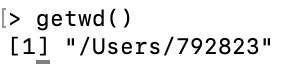
To check the location of the working directory, use the
getwdfunctionOn my MacOS system I get \qquad
![]()
File paths are always enclosed in double quotation marks
Note that R uses forward slashes (not backslashes) for paths
You can change the default working directory using the function
setwd
- File path can be relative to current working directory or full (system root drive)
Working Directory
RStudio
In RStudio you can set the working directory from the menu bar:
- Session
->Set Working Directory->Choose Directory
R Packages
- The base installation of R comes ready with:
- Commands for numeric calculations
- Common statistical analyses
- Plotting and visualization
- More specialized techniques and data sets are contained in packages (libraries)
Help!
- R comes with help files that you can use to search for particular functionality
- For example you can check out how to precisely use a given function
- To call for help type
help(object_name)
Further Help
- Sometimes the output of
help()can be cryptic - Seek help through Google
- Qualify the search with R or the name of an R package
- Paste an error message – chances are it is common error
- Even better: Internet search sites specialized for R searches
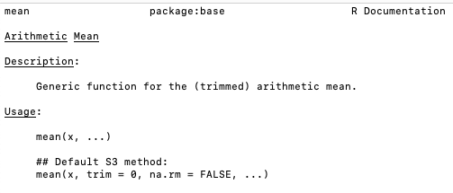
Plotting random numbers
Let us go back to the example of the command plot(rnorm(1000))
The function rnorm(n) outputs n randomly generated numbers from N(0,1)
These can then be plotted by concatenating the plot command
Note:
The values plotted (next slide) are, for sure, different from the ones listed above
This is because every time you call
rnorm(5)new values are generatedWe need to store the generated values if we want to re-use them
Plotting random numbers
Variables and Assignments
- Values can be stored in symbolic variables or objects
- To store values into variables we use assignments
- The assignment operator in R is denoted by
<- <-denotes an arrow pointing to the variable to which the value is assigned
Variables and Assignments
Example
- To assign the value
2to the variablexenterx <- 2 - To recover the value in
xjust typex
Variables and Assignments
Example
- From now on,
xhas the value2 - The variable
xcan be used in subsequent operations - Such operations do not alter the value of
x
Print and Cat
If you save the following code in a
.Rfile and run it, you will obtain no outputThis is because you need to tell R to print
xto screen
- To print a variable to screen use the function
print()
[1] 2Print and Cat
- Suppose you wish to print the sentence Stats is great! to screen
- To do this, we need to store this sentence in a string
- A string is just a sequence of characters enclosed by:
- double-quotations marks
- or single quotations marks
Print and Cat
- If now we wish to print the string
sentenceto screen we can use
- To avoid R displaying the quotation marks, we can instead use
cat()
Print and Cat
catcan be used to combine strings and variables in a single output
Example - Your first R code
- Open a text editor and copy paste the below code
Example - Your first R code
Save to a plain text file named either
my_first_code.Rmy_first_code.txt
Move this file to Desktop
Open the R Console and change working directory to Desktop
Example - Your first R code
- Run your code in the R Console by typying either
- You should get the following output
Code run successfully!The sum of 1 and 2 is 3The workspace
- Variables created in a session are stored in a Workspace
- To display stored variables use
ls()
The workspace
You can remove variables from workspace by using
rm()
The workspace
To completely clear the workspace use
rm(list = ls())
Saving the Workspace
- You can save the workspace using the command
save.image("file_name.RData")
- The file
file_name.RData- Is saved in the working directory
- Contains all the objects currently in the workspace
- You can load a saved workspace in a new R session with the command
load("file_name.RData")
Project Management
Recommended: keep all the files related to a project in a single folder
Such folder will have to be set as working directory in R Console
Saving the workspace could be dangerous
- This is because R Console automatically loads existing saved workspaces
- You might forget that this happens, and have undesired objects in workspace
- This might lead to unintended results
Always store your code in R Scripts
Exiting R and Saving
To quit the R Console type q()
- You will be asked if you want to save your session
- If you say YES, the session will be saved in a
.RDatafile in the working directory - Such file will be automatically loaded when you re-open the R Console
- I recommend you DO NOT save your session
Exiting R and Saving
Summary
- Write your code in R Scripts
- These are
.txtor.Rtext files - For later: Data should be stored in
.txtfiles - DO NOT save your session when prompted
Part 3:
Vectors
Vectors
- We saw how to store a single value in a variable
- Series of values can be stored in vectors
- Vectors can be constructed via the command
c()
Vectorized arithmetic
- A vector is handled by R as a single object
- You can do calculations with vectors, as long as they are of the same length
- Important: Operations are exectuted component-wise
# Constuct two vectors of radius and height of 6 cylinders
radius <- c(6, 7, 5, 9, 9, 7)
height <- c(1.7, 1.8, 1.6, 2, 1, 1.9)

# Compute the volume of each cylinder and store it in "volume"
volume <- pi * radius^2 * height

# Print volume
print(volume)
[1] 192.2655 277.0885 125.6637 508.9380 254.4690 292.4823Vectorized arithmetic
- If 2 vectors do not have the same length then the shorter vector is cycled
- This is called broadcasting
- In the example the vector
ahas 7 components whilebhas 2 components - The operation
a + bis executed as follows:bis copied 4 times to match the length ofaa + bis then obtained by a + \tilde{b} = (1, 2, 3, 4, 5, 6, 7) + (0, 1, 0, 1, 0, 1, 0) = (1, 3, 3, 5, 5, 7, 7)
Vectorized arithmetic
Useful applications of broadcasting are:
- Multiplying a vector by a scalar
- Adding a scalar to each component of a vector
Sum and length
Two very useful vector operators are:
sum(x)which returns the sum of the components ofxlength(x)which returns the length ofx
x <- c(1, 2, 3, 4, 5)

sum <- sum(x)
length <- length(x)

cat("Here is the vector x:", x)
cat("The components of vector x sum to", sum)
cat("The length of vector x is", length)
Here is the vector x: ( 1 2 3 4 5 )The components of vector x sum to 15The length of vector x is 5Computing sample mean and variance
Using vectorized operations
Given a vector \mathbf{x}= (x_1,\ldots,x_n) we want to compute sample mean and variance \overline{x} = \frac{1}{n} \sum_{i=1}^n x_i \,, \qquad s^2 = \frac{\sum_{i=1}^n (x_i - \overline{x})^2 }{n-1}
Computing sample mean and variance
Using built in functions
- R is a statistical language
- There are built in functions to compute sample mean and variance:
mean(x)computes the sample mean ofxsd(x)computes the sample standard deviation ofxvar(x)computes the sample variance ofx
Computing sample mean and variance
Example
- Let us go back to an Example we saw in Lecure 3
- Below is the Wage data on 10 Advertising Professionals Accountants
| Professional | x_1 | x_2 | x_3 | x_4 | x_5 | x_6 | x_7 | x_8 | x_9 | x_{10} |
|---|---|---|---|---|---|---|---|---|---|---|
| Wage | 36 | 40 | 46 | 54 | 57 | 58 | 59 | 60 | 62 | 63 |
- In Lecture 3 we have computed \overline{x} and s^2 by hand
- Let us compute them using R
Computing sample mean and variance
Example
# First store the wage data into a vector
x <- c(36, 40, 46, 54, 57, 58, 59, 60, 62, 63)

# Compute the sample mean using formula
xbar = sum(x) / length(x)

# Compute the sample mean using built in R function
xbar_check = mean(x)

# We now print both results to screen
cat("Sample mean computed with formula is", xbar)
cat("Sample mean computed by R is", xbar_check)
cat("They coincide!")
Sample mean computed with formula is 53.5Sample mean computed by R is 53.5They coincide!Computing sample mean and variance
Example
# Compute the sample variance using formula
xbar = mean(x)
n = length(x)
s2 = sum( (x - xbar)^2 ) / (n - 1)

# Compute the sample variance using built in R function
s2_check = var(x)

# We now print both results to screen
cat("Sample variance computed with formula is", s2)
cat("Sample variance computed by R is", s2_check)
cat("They coincide!")
Sample variance computed with formula is 90.27778Sample variance computed by R is 90.27778They coincide!Part 4:
t-test in R
t-test in R
- We are now ready to do some statistics in R
- We start by looking at the t-test
- Specifically, to the One-sample Two-sided t-test
Goal of t-test: Estimate mean \mu of normal population N(\mu,\sigma^2). If \mu_0 is guess for \mu H_0 \colon \mu = \mu_0 \qquad H_1 \colon \mu \neq \mu_0
Method: Given sample X_1 ,\ldots,X_n we look at the statistics T = \frac{\overline{X}-\mu_0}{S/\sqrt{n}} \sim t_{n-1}
t-test by hand
Given the data x_1,\ldots,x_n, compute the t-statistic t = \frac{\text{estimate } - \text{ hypothesised value}}{\mathop{\mathrm{e.s.e.}}} = \frac{\overline x - \mu_0}{s/\sqrt{n}} with sample mean and sample standard deviation \overline{x} = \frac{1}{n} \sum_{i=1}^n x_i \,, \qquad s = \sqrt{\frac{\sum_{i=1}^n x_i^2 - n \overline{x}^2}{n-1}}
Find the critical value t^* = t_{n-1}(0.025) in Statistical Table 13.1
- If |t|>t^* reject H_0. The mean is not \mu_0
- If |t| \leq t^* do not reject H_0. There is not enough evidence
t-test
Given the sample x_1,\ldots,x_n, R can compute the t-statistic t = \frac{\text{estimate } - \text{ hypothesised value}}{\mathop{\mathrm{e.s.e.}}} = \frac{\overline x - \mu_0}{s/\sqrt{n}}
R can compute the precise p-value (no need for Statistical Tables) p = 2P(|t_{n-1}|>t)
- If p < 0.05 reject H_0. The mean is not \mu_0
- If p \geq 0.05 do not reject H_0. There is not enough evidence
Note: The above operations can be done at the same time by command t.test
t-test code in R
- Store the sample x_1,\ldots,x_n in an R vector using
data_vector <- c(x1, ..., xn)
- Perform a two-sided t-test on
data_vectorwith null hypothesismu0usingt.test(data_vector, mu = mu0)
- Read output. R will tell you
- t-statistic
- degrees of freedom
- p-value
- alternative hypothesis
- confidence interval (where true mean is likely to be)
- sample mean
t-test command
Relevant options of t.test are
mu = mu0tells R to test null hypothesis H_0 \colon \mu = \mu_0If
mu = mu0is not specified, R assumes \mu_0 = 0alternative = "greater"tells R to perform one-sided t-test H_0 \colon \mu > \mu_0
t-test command
alternative = "smaller"tells R to perform one-sided t-test H_0 \colon \mu < \mu_0conf.level = nchanges the confidence interval level ton(default is 0.95)
Example: 2008 crisis
Let us go back to the 2008 Crisis example
- Data: Monthly Consumer Confidence Index (CCI) in 2007 and 2009
- Question: Did the crash of 2008 have lasting impact upon CCI?
- Observation: Data shows a massive drop in CCI between 2009 and 2007
- Method: Use t-test to see if data is sufficient to prove that CCI actually dropped
| Month | J | F | M | A | M | J | J | A | S | O | N | D |
|---|---|---|---|---|---|---|---|---|---|---|---|---|
| CCI 2007 | 86 | 86 | 88 | 90 | 99 | 97 | 97 | 96 | 99 | 97 | 90 | 90 |
| CCI 2009 | 24 | 22 | 21 | 21 | 19 | 18 | 17 | 18 | 21 | 23 | 22 | 21 |
| Difference | 62 | 64 | 67 | 69 | 80 | 79 | 80 | 78 | 78 | 74 | 68 | 69 |
Example: 2008 crisis
Setting up the test
We want to test if there was a change in CCI from 2007 to 2009
We interested in the difference in CCI
The null hypothesis is that there was (on average) no change in CCI H_0 \colon \mu = 0
The alternative hypothesis is that there was some change: H_1 \colon \mu \neq 0
Example: 2008 crisis
R code
# Enter CCI data in 2 vectors using function c()
score_2007 <- c(86, 86, 88, 90, 99, 97, 97, 96, 99, 97, 90, 90)
score_2009 <- c(24, 22, 21, 21, 19, 18, 17, 18, 21, 23, 22, 21)

# Compute vector of differences in CCI
difference <- score_2007 - score_2009

# Perform t-test on difference with null hypothesis mu = 0
# Store answer in "answer"
answer -> t.test(difference, mu = 0)

# Print the answer
print(answer)- Code can be downloaded here one_sample_t_test.R
Example: 2008 crisis
Output of t.test
    One Sample t-test

data:  difference
t = 38.144, df = 11, p-value = 4.861e-13
alternative hypothesis: true mean is not equal to 0
95 percent confidence interval:
 68.15960 76.50706
sample estimates:
mean of x
 72.33333
Example: 2008 crisis
Analysis of Output
One Sample t-test- Description of the test that we have asked for
- Note:
t.testhas automatically assumed that a one-sample test is desired
Example: 2008 crisis
Analysis of Output
data: difference- This says which data are being tested
- In our case we test the data in
difference
Example: 2008 crisis
Analysis of Output
t = 38.144, df = 11, p-value = 4.861e-13This is the best part:
- \texttt{t} = \, t-statistic from data
- \texttt{df} = \, degrees of freedom
- \texttt{p-value} = \, the exact p-value
Note:
- You do not need Statistical Tables!
- You see that p < 0.05
- Therefore we reject null hypothesis that the mean difference is 0
Example: 2008 crisis
Analysis of Output
alternative hypothesis: true mean is not equal to 0R tells us the alternative hypothesis is \mu \neq 0
Hence the Null hypothesis tested is H_0 \colon \mu = 0
Warning:
- This message is not telling you to accept to alternative hypothesis
- This message is only stating the alternative hypothesis
Example: 2008 crisis
Analysis of Output
95 percent confidence interval: 68.15960 76.50706This is a 95 \% confidence interval for the true mean:
- Confidence interval: is the set of (hypothetical) mean values from which the data do not deviate significantly
- It is based on inverting the t-test by solving for the values of \mu that cause t to lie within its acceptance region
Example: 2008 crisis
Analysis of Output
95 percent confidence interval: 68.15960 76.50706- For 95 \% confidence interval this means solving P( |t_{n-1}| < t) = 0.95 \,, \qquad t = \frac{\overline{x}-\mu}{\mathop{\mathrm{e.s.e.}}}
- Solving wrt \mu yields \overline{x} - t_{n-1}(0.025) \times \mathop{\mathrm{e.s.e.}}< \mu < \overline{x} + t_{n-1}(0.025) \times \mathop{\mathrm{e.s.e.}}
Example: 2008 crisis
Analysis of Output
95 percent confidence interval: 68.15960 76.50706R calculated the quantities \overline{x} \pm t_{n-1}(0.025) \times \mathop{\mathrm{e.s.e.}}
Based on the data, we conclude that the set of (hypothetical) mean values is \mu \in [68.15960, 76.50706]
Example: 2008 crisis
Analysis of Output
sample estimates:mean of x 72.33333 - This is the sample mean
- You could have easily computed this with the code
mean(difference)
Example: 2008 crisis
Conclusion
The key information is:
- We conducted a two-sided t-test for the mean difference \mu \neq 0
- Results give significant evidence p<0.05 that \mu \neq 0
- The sample mean difference \overline{x} = 72.33333 \gg 0
- This suggest CCI mean difference \mu \gg 0
- Hence consumer confidence is higher in 2007 than in 2009
Part 5:
Graphics
Graphics
R has extensive built in graphing functions:
Fancier graphing functions are contained in the library
ggplot2(see link)However we will be using the basic built in R graphing functions
Graphics
Scatter plot
- Suppose given 2 vectors
xandyof same length - The scatter plot of pairs (x_i,y_i) can be generated with
plot(x, y)
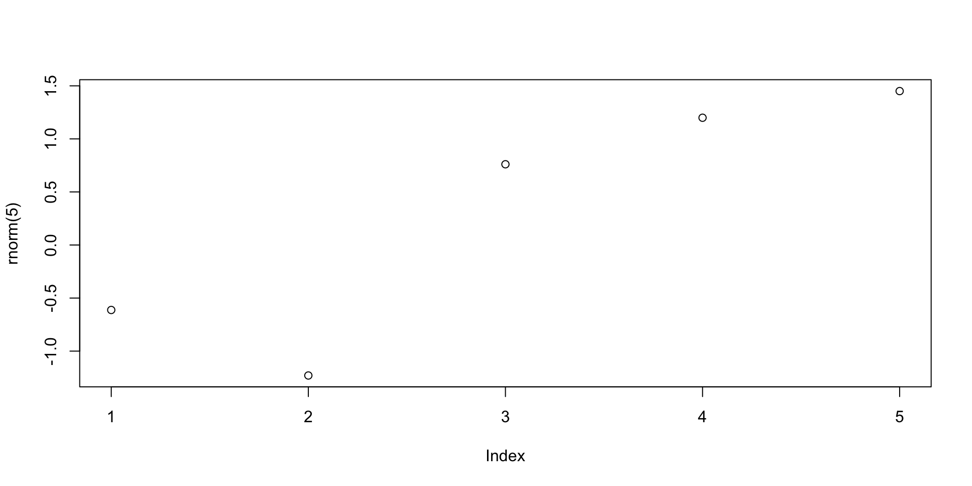
Example: Suppose to have data of weights and heights of 6 people
- To plot weight against height code is as follows
- When you run
plot()in R Console the plot will appear in a pop-up window
Graphics
Graphics
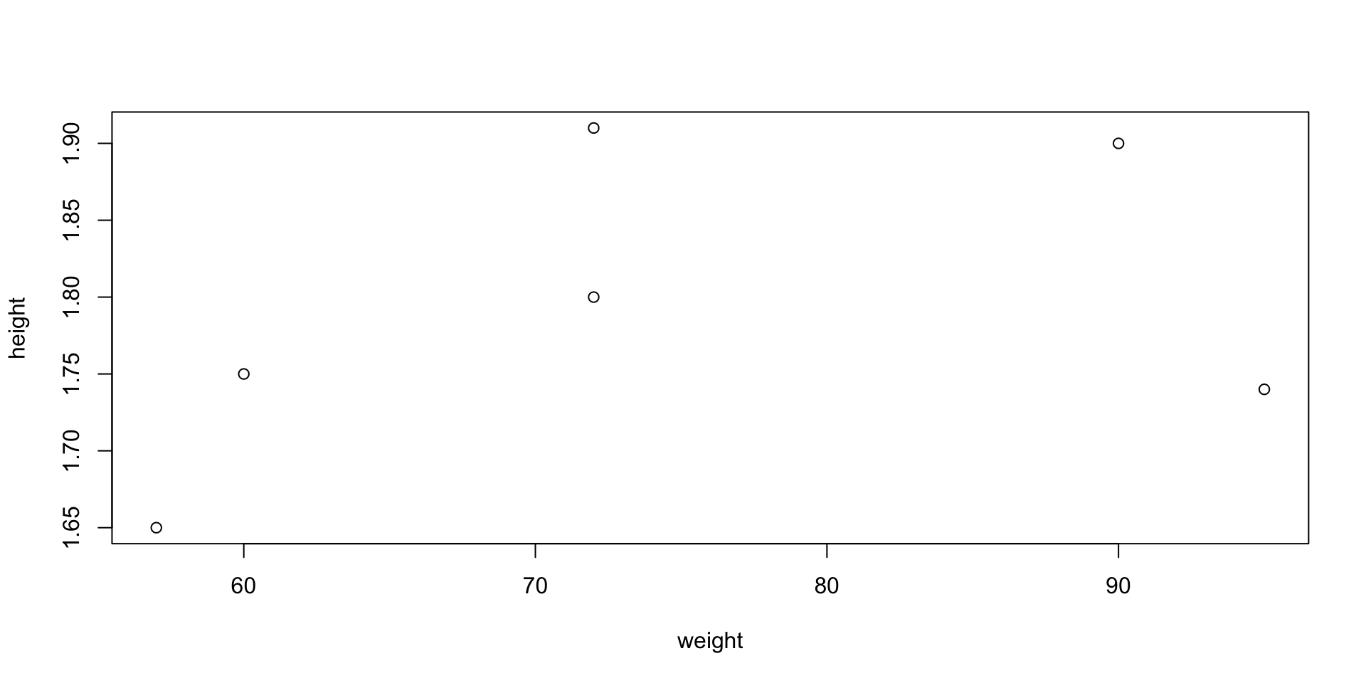
Scatter plot – Options
- You can customize your plot in many ways
- Example: you can represent points (x_i,y_i) with triangles instead of circles
- This can be done by including the command
pch = 2
pchstands for plotting character
Graphics
Graphics
Plotting 1D function f(x)
- Create a grid of x values x = (x_1, \ldots, x_n)
- Evaluate f on such grid. This yields a vector y = (f(x_1), \ldots, f(x_n))
- Generate a scatter plot with
plot(x, y)
- Use the function
linesto linearly interpolate the scatter plot:lines(x, y)
Graphics
Plotting functions - Example
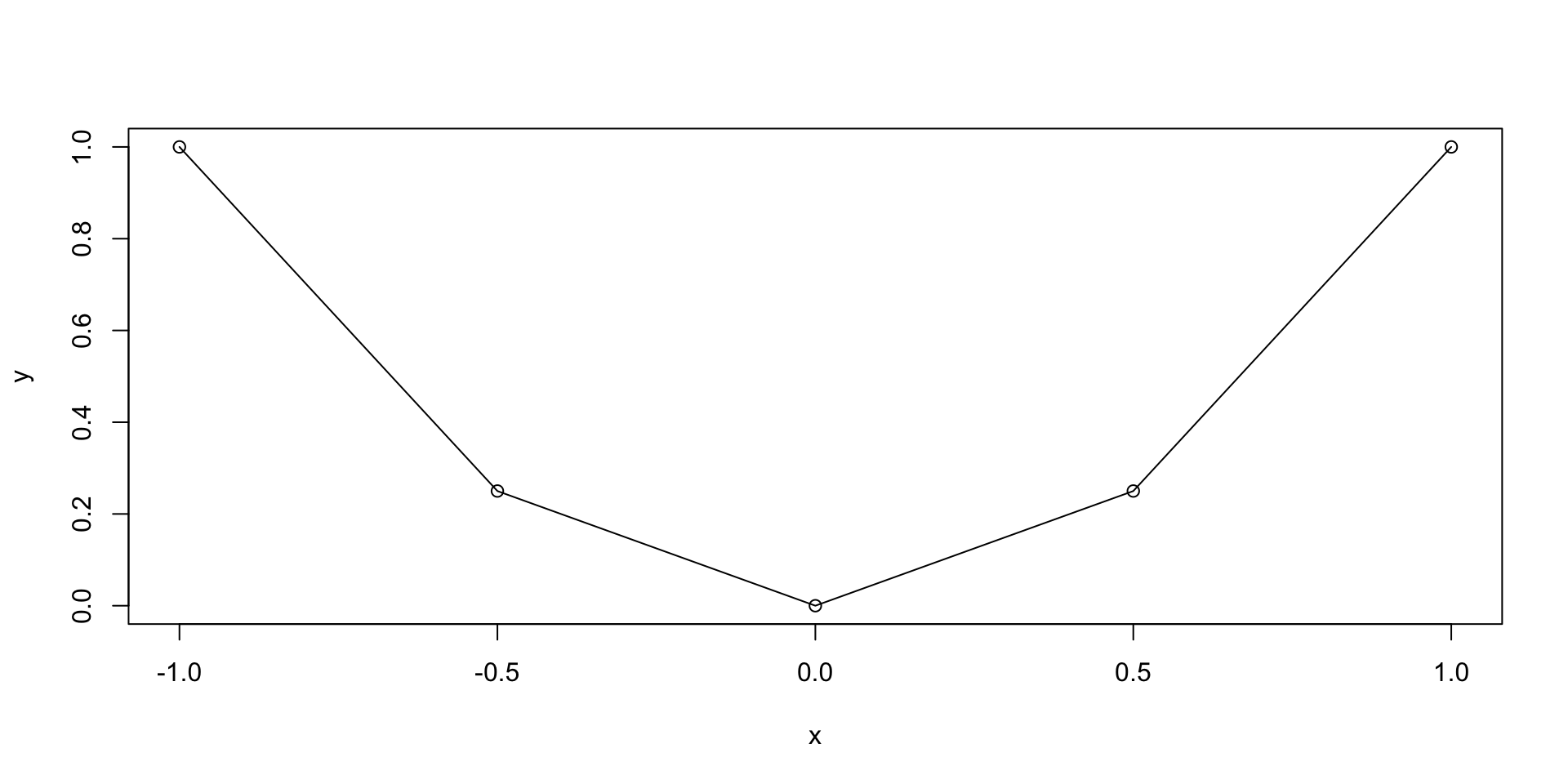
Let us plot the parabola y = x^2 \,, \qquad x \in [-1,1]
Graphics
Graphics
Plotting functions - Example
The previous plot was quite rough
This is because we only computed y=x^2 on the grid x = (-1, -0.5, 0, 0.5, 1)
We could refine the grid by hand, but this is not practical
To generate a finer grid we can use the built in R function
seq()
Seq function
seq(from, to, by, length.out) generates a vector containing a sequence:
from– The beginning number of the sequenceto– The ending number of the sequenceby– The step-size of the sequence (the increment)length.out– The total length of the sequence
Example: Generate the vector of even numbers from 2 to 20
Seq function
Note: The following commands are equivalent:
seq(from = x1, to = x2, by = s)seq(x1, x2, s)
Example: Generate the vector of odd numbers from 1 to 11
x <- seq(from = 1, to = 11, by = 2)
y <- seq(1, 11, 2)

cat("Vector x is: (", x, ")")
cat("Vector y is: (", y, ")")
cat("They are the same!")
Vector x is: ( 1 3 5 7 9 11 )Vector y is: ( 1 3 5 7 9 11 )They are the same!Graphics
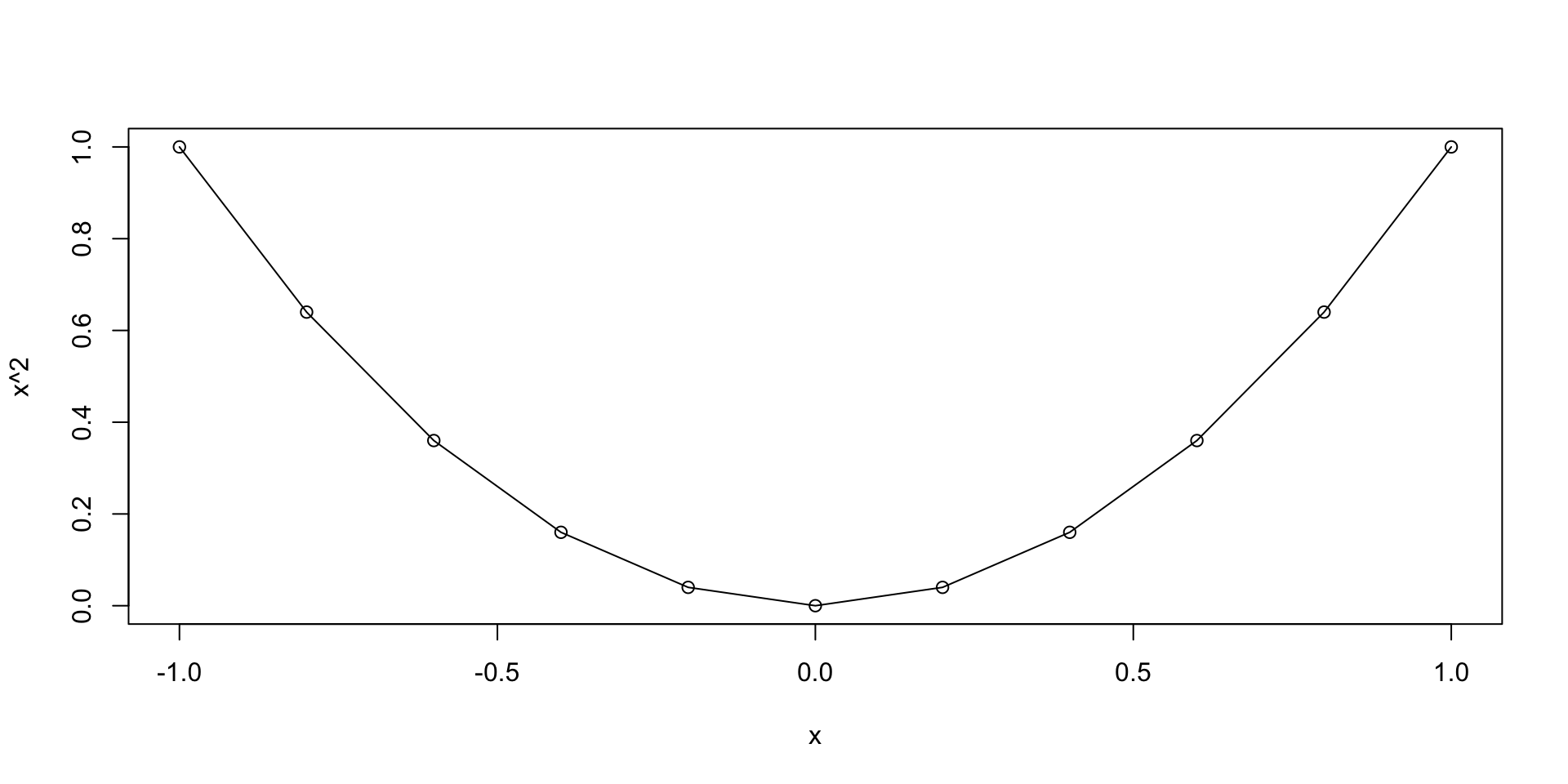
Plotting functions - Example
- We go back to plotting y = x^2 \,, \qquad x \in [-1, 1]
- We want to generate a grid, or sequece:
- Starting at 0
- Ending at 1
- With increments of 0.2
Graphics
Plotting functions - Example
Graphics
Scatter plot - Example
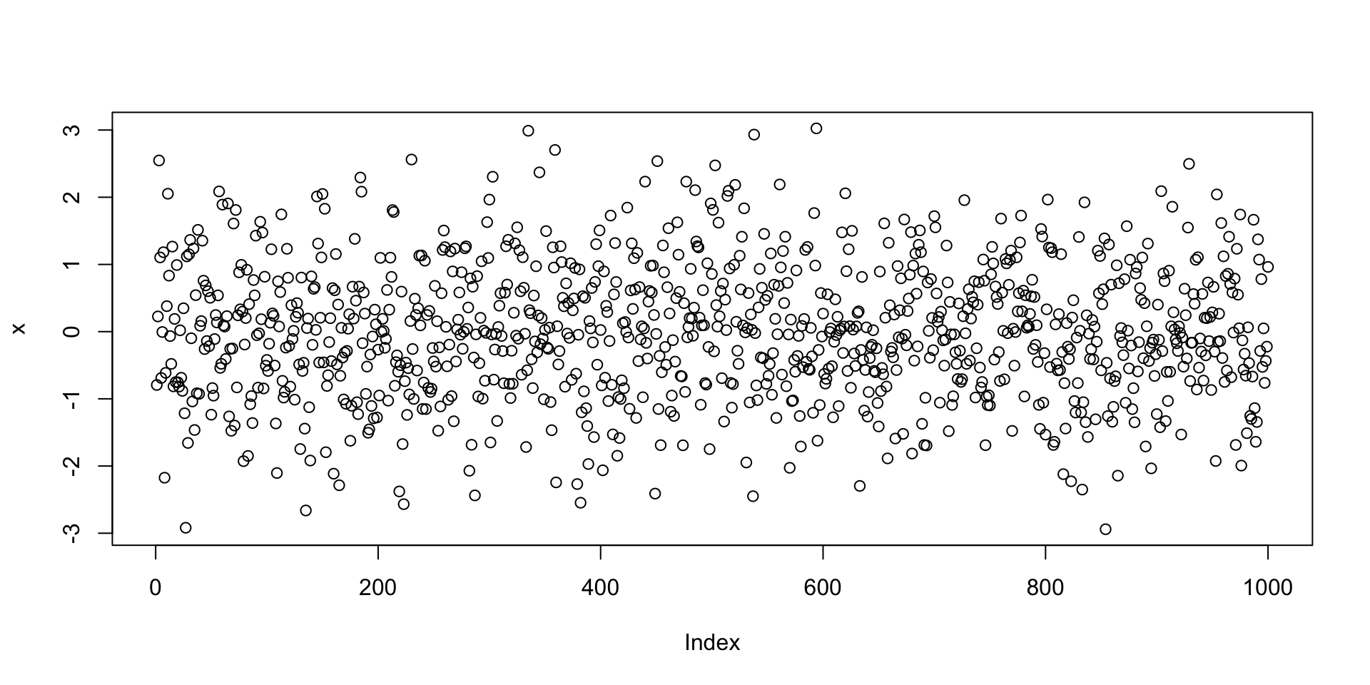
Let us go back to the example of plotting random normal values
- First we generate a vector
xwith 1000 random normal values - Then we plot
xviaplot(x) - The command
plot(x)implicitly assumes that:xis the second argument: Values to plot on y-axis- The first argument is the vector
seq(1, 1000) - Note that
seq(1, 1000)is the vector of components numbers ofx
Graphics
References
[1]
Dalgaard, Peter, Introductory statistics with R, Second Edition, Springer, 2008.
[2]
Davies, Tilman M., The book of R, No Starch Press, 2016.
Comments
#