Statistical Models
Lecture 2
Lecture 2:
Multivariate distributions
Outline of Lecture 2
- Bivariate random vectors
- Conditional distributions
- Independence
- Covariance and correlation
- Multivariate random vectors
Univariate vs Bivariate vs Multivariate
- Probability models seen so far only involve 1 random variable
- These are called univariate models
- We are also interested in probability models involving multiple variables:
- Models with 2 random variables are called bivariate
- Models with more than 2 random variables are called multivariate
Random vectors
Definition
Recall: a random variable is a measurable function X \colon \Omega \to \mathbb{R}\,, \quad \Omega \,\, \text{ sample space}
Definition
A random vector is a measurable function \mathbf{X}\colon \Omega \to \mathbb{R}^n. We say that
- \mathbf{X} is univariate if n=1
- \mathbf{X} is bivariate if n=2
- \mathbf{X} is multivariate if n \geq 3
Random vectors
Notation
The components of a random vector \mathbf{X} are denoted by \mathbf{X}= (X_1, \ldots, X_n) with X_i \colon \Omega \to \mathbb{R} random variables
We denote a two-dimensional bivariate random vector by (X,Y) with X,Y \colon \Omega \to \mathbb{R} random variables
Part 1:
Bivariate random vectors
Discrete random vectors
Main definitions
Definition
The (bivariate) random vector (X,Y) is discrete if X and Y are discrete random variables
Definition
The joint probability mass function or joint pmf of a discrete random vector (X,Y) is the function f_{X,Y} \colon \mathbb{R}^2 \to \mathbb{R} defined by
f_{X,Y}(x,y) := P( \{X=x \} \cap \{ Y=y \}) \,, \qquad \forall \, (x,y) \in \mathbb{R}^2
Notation: P(X=x, Y=y ) := P( \{X=x \} \cap \{ Y=y \})
Discrete random vectors
Computing probabilities
The joint pmf can be used to compute the probability of A \subset \mathbb{R}^2 \begin{align*} P((X,Y) \in A) & := P( \{ \omega \in \Omega \colon ( X(\omega), Y(\omega) ) \in A \} ) \\ & = \sum_{(x,y) \in A} f_{X,Y} (x,y) \end{align*}
In particular we obtain \sum_{(x,y) \in \mathbb{R}^2} f_{X,Y} (x,y) = 1
Discrete random vectors
Expected value
- Suppose (X,Y) \colon \Omega \to \mathbb{R}^2 random vector and g \colon \mathbb{R}^2 \to \mathbb{R} function
- Then g(X,Y) \colon \Omega \to \mathbb{R} is random variable
Definition
The expected value of the random variable g(X,Y) is
{\rm I\kern-.3em E}[g(X,Y)] := \sum_{(x,y) \in \mathbb{R}^2} g(x,y) f_{X,Y}(x,y) = \sum_{(x,y) \in \mathbb{R}^2} g(x,y) P(X=x,Y=y)
Discrete random vectors
Marginals
Definition
Let (X,Y) be a discrete random vector. The marginal pmfs of X and Y are the functions
f_X (x) := P(X = x) \quad \text{ and } \quad
f_Y(y) := P(Y = y)
Note: The marginal pmfs of X and Y are just the usual pmfs of X and Y
Discrete random vectors
Marginals
Marginals of X and Y can be computed from the joint pmf f_{X,Y}
Theorem
Let (X,Y) be a discrete random vector with joint pmf f_{X,Y}. The marginal pmfs of X and Y are given by
f_X(x) = \sum_{y \in \mathbb{R}} f_{X,Y}(x,y) \quad \text{ and }
\quad
f_Y(y) = \sum_{x \in \mathbb{R}} f_{X,Y}(x,y)
Example - Discrete random vector
Setting
- Consider experiment of tossing two dice. Then sample space is \Omega = \{ (m,n) \colon m,n \in \{1,\ldots,6\} \} with m and n being the outcomes of first and second dice, respectively
- We assume that the dice are fair. Therefore P(\{(m,n)\})=1/36
- Define the discrete random variables \begin{align*} X(m,n) & := m + n \quad & \text{ sum of the dice} \\ Y(m,n) & := | m - n| \quad & \text{ |difference of the dice|} \end{align*}
- For example X(3,3) = 3 + 3 = 6 \qquad \qquad Y(3,3) = |3 - 3| = 0
Example - Discrete random vector
Computing joint pmf
To compute joint pmf one needs to consider all the cases f_{X,Y}(x,y) = P(X=x,Y=y) \,, \quad (x,y) \in \mathbb{R}^2
For example X=4 and Y=0 is only obtained for (2,2). Hence f_{X,Y}(4,0) = P(X=4,Y=0) = P(\{(2,2)\}) = \frac{1}{6} \cdot \frac{1}{6} = \frac{1}{36}
Similarly X=5 and Y=2 is only obtained for (4,1) and (1,4). Thus f_{X,Y}(5,2) = P(X=5,Y=2) = P(\{(4,1)\} \cup \{(1,4)\}) = \frac{1}{36} + \frac{1}{36} = \frac{1}{18}
Example - Discrete random vector
Computing joint pmf
f_{X,Y}(x,y)=0 for most of the pairs (x,y). Indeed f_{X,Y}(x,y)=0 if x \notin X(\Omega) \quad \text{ or } \quad y \notin Y(\Omega)
We have X(\Omega)=\{2,3,4,5,6,7,8,9,10,11,12\}
We have Y(\Omega)=\{0,1,2,3,4,5\}
Hence f_{X,Y} only needs to be computed for pairs (x,y) satisfying 2 \leq x \leq 12 \quad \text{ and } \quad 0 \leq y \leq 5
Within this range, other values will be zero. For example f_{X,Y}(3,0) = P(X=3,Y=0) = P(\emptyset) = 0
Example - Discrete random vector
Table of values of joint pmf
Below are all the values for f_{X,Y}. Empty entries correspond to f_{X,Y}(x,y) = 0
| x | ||||||||||||
|---|---|---|---|---|---|---|---|---|---|---|---|---|
| 2 | 3 | 4 | 5 | 6 | 7 | 8 | 9 | 10 | 11 | 12 | ||
| 0 | 1/36 | 1/36 | 1/36 | 1/36 | 1/36 | 1/36 | ||||||
| 1 | 1/18 | 1/18 | 1/18 | 1/18 | 1/18 | |||||||
| y | 2 | 1/18 | 1/18 | 1/18 | 1/18 | |||||||
| 3 | 1/18 | 1/18 | 1/18 | |||||||||
| 4 | 1/18 | 1/18 | ||||||||||
| 5 | 1/18 |
Example - Discrete random vector
Expected value
- We want to compute {\rm I\kern-.3em E}[XY]
- Hence consider the function g(x,y):=xy
- We obtain \begin{align*} {\rm I\kern-.3em E}[XY] & = {\rm I\kern-.3em E}[g(X,Y)] \\ & = \sum_{(x,y) \in \mathbb{R}^2} g(x,y) f_{X,Y}(x,y)\\ & = \sum_{(x,y) \in \mathbb{R}^2} xy f_{X,Y}(x,y) \end{align*}
Example - Discrete random vector
Expected value
We can use the non-zero entries in the table for f_{X,Y} to compute: \begin{align*} {\rm I\kern-.3em E}[XY] & = 3 \cdot 1 \cdot \frac{1}{18} + 5 \cdot 1 \cdot \frac{1}{18} + 7 \cdot 1 \cdot \frac{1}{18} + 9 \cdot 1 \cdot \frac{1}{18} + 11 \cdot 1 \cdot \frac{1}{18} \\ & + 4 \cdot 2 \cdot \frac{1}{18} + 6 \cdot 2 \cdot \frac{1}{18} + 8 \cdot 2 \cdot \frac{1}{18} + 10\cdot 2 \cdot \frac{1}{18} \\ & + 5 \cdot 3 \cdot \frac{1}{18} + 7 \cdot 3 \cdot \frac{1}{18} + 9 \cdot 3 \cdot \frac{1}{18} \\ & + 6 \cdot 4 \cdot \frac{1}{18} + 8 \cdot 4 \cdot \frac{1}{18} \\ & + 7 \cdot 5 \cdot \frac{1}{18} \\ & = (35 + 56 + 63 + 56 + 35 ) \frac{1}{18} = \frac{245}{18} \end{align*}
Example - Discrete random vector
Marginals
We want to compute the marginal of Y via the formula f_Y(y) = \sum_{x \in \mathbb{R}} f_{X,Y}(x,y)
Again looking at the table for f_{X,Y}, we get \begin{align*} f_Y(0) & = f_{X,Y}(2,0) + f_{X,Y}(4,0) + f_{X,Y}(6,0) \\ & + f_{X,Y}(8,0) + f_{X,Y}(10,0) + f_{X,Y}(12,0) \\ & = 6 \cdot \frac{1}{36} = \frac{3}{18} \end{align*}
Example - Discrete random vector
Marginals
- Similarly, we get \begin{align*} f_Y(1) & = f_{X,Y}(3,1) + f_{X,Y}(5,1) + f_{X,Y}(7,1) \\ & + f_{X,Y}(9,1) + f_{X,Y}(11,1) \\ & = 5 \cdot \frac{1}{18} = \frac{5}{18} \end{align*}
- And the remaining values follow a similar pattern: f_Y(2) = \frac{4}{18} \,, \quad f_Y(3) = \frac{3}{18} \,, \quad f_Y(4) = \frac{2}{18} \,, \quad f_Y(5) = \frac{1}{18} \,, \quad
Example - Discrete random vector
Marginals
Hence the pmf of Y is given by the table below
| y | 0 | 1 | 2 | 3 | 4 | 5 |
|---|---|---|---|---|---|---|
| f_Y(y) | \frac{3}{18} | \frac{5}{18} | \frac{4}{18} | \frac{3}{18} | \frac{2}{18} | \frac{1}{18} |
Note that f_Y is indeed a pmf, since \sum_{y \in \mathbb{R}} f_Y(y) = \sum_{y=0}^5 f_Y(y) = 1
Continuous random vectors
Definition
The random vector (X,Y) is continuous if X and Y are continuous rv
Definition
The joint probability density function or joint pdf of a continuous random vector (X,Y) is a function f_{X,Y} \colon \mathbb{R}^2 \to \mathbb{R} s.t.
P((X,Y) \in A) = \int_{A} f_{X,Y}(x,y) \, dxdy
- \int_A is a double integral over A, like the ones you saw in Calculus
- The joint pdf is defined over the whole \mathbb{R}^2
Continuous random vectors
Expected value
- Suppose (X,Y) \colon \Omega \to \mathbb{R}^2 continuous random vector and g \colon \mathbb{R}^2 \to \mathbb{R} function
- Then g(X,Y) \colon \Omega \to \mathbb{R} is random variable
Definition
The expected value of the random variable g(X,Y) is
{\rm I\kern-.3em E}[g(X,Y)] := \int_{\mathbb{R}^2} g(x,y) f_{X,Y}(x,y) \, dxdy
Notation:The symbol \int_{\mathbb{R}^2} denotes the double integral \int_{-\infty}^\infty\int_{-\infty}^\infty
Continuous random vectors
Marginals
Definition
Let (X,Y) be a continuous random vector. The marginal pdfs of X and Y are functions f_X,f_Y \colon \mathbb{R}\to \mathbb{R} s.t.
P(a \leq X \leq b) = \int_{a}^b f_X (x) \,dx \quad \text{ and } \quad
P(a \leq Y \leq b) = \int_{a}^b f_Y (y) \,dy
Note: The marginal pdfs of X and Y are just the usual pdfs of X and Y
Continuous random vectors
Marginals
Marginals of X and Y can be computed from the joint pdf f_{X,Y}
Theorem
Let (X,Y) be a discrete random vector with joint pdf f_{X,Y}. The marginal pdfs of X and Y are given by
f_X(x) = \int_{-\infty}^\infty f_{X,Y}(x,y) \,dy \quad \text{ and }
\quad
f_Y(y) = \int_{-\infty}^\infty f_{X,Y}(x,y) \, dx
Characterization of joint pmf and pdf
Theorem
Let f \colon \mathbb{R}^2 \to \mathbb{R}. Then f is joint pmf or joint pdf of a random vector (X,Y) iff
- f(x,y) \geq 0 for all (x,y) \in \mathbb{R}^2
- \sum_{(x,y) \in \mathbb{R}^2} f(x,y) = 1 \,\,\, (joint pmf) \quad or \quad \int_{\mathbb{R}^2} f(x,y) \,dxdy = 1 \,\,\, (joint pdf)
In the above setting:
- The random vector (X,Y) has distribution
- P(X=x,Y=y ) = f(x,y) \,\,\,\text{ (joint pmf)}
- P((X,Y) \in A) = \int_A f (x,y) \, dxdy \,\,\, \text{ (joint pdf)}
- The symbol (X,Y) \sim f denotes that (X,Y) has distribution f
Summary - Random Vectors
| (X,Y) discrete random vector | (X,Y) continuous random vector |
|---|---|
| X and Y discrete | X and Y continuous |
| Joint pmf | Joint pdf |
| f_{X,Y}(x,y) := P(X=x,Y=y) | P((X,Y) \in A) = \int_A f_X(x,y) \,dxdy |
| f_{X,Y} \geq 0 | f_{X,Y} \geq 0 |
| \sum_{(x,y)\in \mathbb{R}^2} f_{X,Y}(x,y)=1 | \int_{\mathbb{R}^2} f_{X,Y}(x,y) \, dxdy= 1 |
| Marginal pmfs | Marginal pdfs |
| f_X (x) := P(X=x) | P(a \leq X \leq b) = \int_a^b f_X(x) \,dx |
| f_Y (y) := P(Y=y) | P(a \leq Y \leq b) = \int_a^b f_Y(y) \,dy |
| f_X (x)=\sum_{y \in \mathbb{R}} f_{X,Y}(x,y) | f_X(x) = \int_{\mathbb{R}} f_{X,Y}(x,y) \,dy |
| f_Y (y)=\sum_{x \in \mathbb{R}} f_{X,Y}(x,y) | f_Y(y) = \int_{\mathbb{R}} f_{X,Y}(x,y) \,dx |
Linearity of Expected Value
Theorem
(X,Y) random vector, g,h \colon \mathbb{R}^2 \to \mathbb{R} functions and a,b,c \in \mathbb{R}. The expectation is linear: \begin{equation} \tag{1}
{\rm I\kern-.3em E}( a g (X,Y) + b h(X,Y)+ c ) = a {\rm I\kern-.3em E}[g(X,Y)] + b {\rm I\kern-.3em E}[h(X,Y)] + c
\end{equation} In particular \begin{equation} \tag{2}
{\rm I\kern-.3em E}[a X + b Y] = a{\rm I\kern-.3em E}[X] + b{\rm I\kern-.3em E}[Y]
\end{equation}
- Proof of (1) follows by definition (see also argument in Slide 90 in Lecture 1)
- Equation (2) follows from (1) by setting c=0 \,, \quad g(x,y)=x \,, \qquad h(x,y)=y
Part 2:
Conditional distributions
Conditional distributions - Discrete case
Suppose given a discrete random vector (X,Y)
It might happen that the event \{X=x\} depends on \{Y=y\}
If P(Y=y)>0 we can define the conditional probability P(X=x|Y=y) := \frac{P(X=x,Y=y)}{P(Y=y)} = \frac{f_{X,Y}(x,y)}{f_Y(y)} where f_{X,Y} is joint pmf of (X,Y) and f_Y the marginal pmf of Y
Conditional pmf
Definition
(X,Y) discrete random vector with joint pmf f_{X,Y} and marginal pmfs f_X, f_Y
For any x such that f_X(x)=P(X=x)>0 the conditional pmf of Y given that X=x is the function f(\cdot | x) defined by f(y|x) := P(Y=y|X=x) = \frac{f_{X,Y}(x,y)}{f_X(x)}
For any y such that f_Y(y)=P(X=y)>0 the conditional pmf of X given that Y=y is the function f(\cdot | y) defined by f(x|y) := P(X=x|Y=y) =\frac{f_{X,Y}(x,y)}{f_Y(y)}
Conditional pmf
Conditional pmf f(y|x) is indeed a pmf:
- f(y|x) \geq 0
- \sum_{y} f(y|x) = \dfrac{\sum_{y} f_{X,Y}(x,y)}{f_X(x)} = \dfrac{f_X(x)}{f_X(x)} = 1
- Hence there exists a discrete rv Z whose pmf is f(y|x)
- This is true by the Theorem in Slide 80 in Lecture 1
Similar reasoning yields that also f(x|y) is a pmf
Notation: We will often write
- X|Y to denote the distribution f(x|y)
- Y|X to denote the distribution f(y|x)
Conditional distributions - Continuous case
- In the discrete case we consider the conditional probability P(X=x|Y=y) = \frac{P(X=x,Y=y)}{P(Y=y)}
- However when Y is continuous random variable we have P(Y=y) = 0 \quad \forall \, y \in \mathbb{R}
- Question: How do we define conditional distributions in the continuous case?
- Answer: By replacing pmfs with pdfs
Conditional pdf
Definition
(X,Y) continuous random vector with joint pdf f_{X,Y} and marginal pdfs f_X, f_Y
For any x such that f_X(x)>0 the conditional pdf of Y given that X=x is the function f(\cdot | x) defined by f(y|x) := \frac{f_{X,Y}(x,y)}{f_X(x)}
For any y such that f_Y(y)>0 the conditional pdf of X given that Y=y is the function f(\cdot | y) defined by f(x|y) := \frac{f_{X,Y}(x,y)}{f_Y(y)}
Conditional pdf
- Conditional pdf f(y|x) is indeed a pdf:
- f(y|x) \geq 0
- \int_{y \in \mathbb{R}} f(y|x) \, dy = \dfrac{\int_{y \in \mathbb{R}} f_{X,Y}(x,y) \, dy}{f_X(x)} = \dfrac{f_X(x)}{f_X(x)} = 1
- Hence there exists a continuous rv Z whose pdf is f(y|x)
- This is true by the Theorem in Slide 80 in Lecture 1
- Similar reasoning yields that also f(x|y) is a pdf
Conditional expectation
Definition
(X,Y) random vector and g \colon \mathbb{R}\to \mathbb{R} function. The conditional expectation of g(Y) given X=x is \begin{align*}
{\rm I\kern-.3em E}[g(Y) | x] & := \sum_{y} g(y) f(y|x) \quad \text{ if } (X,Y) \text{ discrete} \\
{\rm I\kern-.3em E}[g(Y) | x] & := \int_{y \in \mathbb{R}} g(y) f(y|x) \, dy \quad \text{ if } (X,Y) \text{ continuous}
\end{align*}
- {\rm I\kern-.3em E}[g(Y) | x] is a real number for all x \in \mathbb{R}
- {\rm I\kern-.3em E}[g(Y) | X] denotes the Random Variable h(X) where h(x):={\rm I\kern-.3em E}[g(Y) | x]
Conditional variance
Definition
(X,Y) random vector. The conditional variance of Y given X=x is
{\rm Var}[Y | x] := {\rm I\kern-.3em E}[Y^2|x] - {\rm I\kern-.3em E}[Y|x]^2
- {\rm Var}[Y | x] is a real number for all x \in \mathbb{R}
- {\rm Var}[Y | X] denotes the Random Variable {\rm Var}[Y | X] := {\rm I\kern-.3em E}[Y^2|X] - {\rm I\kern-.3em E}[Y|X]^2
Example - Conditional distribution
- Continuous random vector (X,Y) with joint pdf f_{X,Y}(x,y) := e^{-y} \,\, \text{ if } \,\, 0 < x < y \,, \quad f_{X,Y}(x,y) :=0 \,\, \text{ otherwise}
Example - Conditional distribution
- We compute f_X, the marginal pdf of X:
- If x \leq 0 then f_{X,Y}(x,y)=0. Therefore f_X(x) = \int_{-\infty}^\infty f_{X,Y}(x,y) \, dy = 0
- If x > 0 then f_{X,Y}(x,y)=e^{-y} if y>x, and f_{X,Y}(x,y)=0 if y \leq x. Thus \begin{align*} f_X(x) & = \int_{-\infty}^\infty f_{X,Y}(x,y) \, dy = \int_{x}^\infty e^{-y} \, dy \\ & = - e^{-y} \bigg|_{y=x}^{y=\infty} = -e^{-\infty} + e^{-x} = e^{-x} \end{align*}
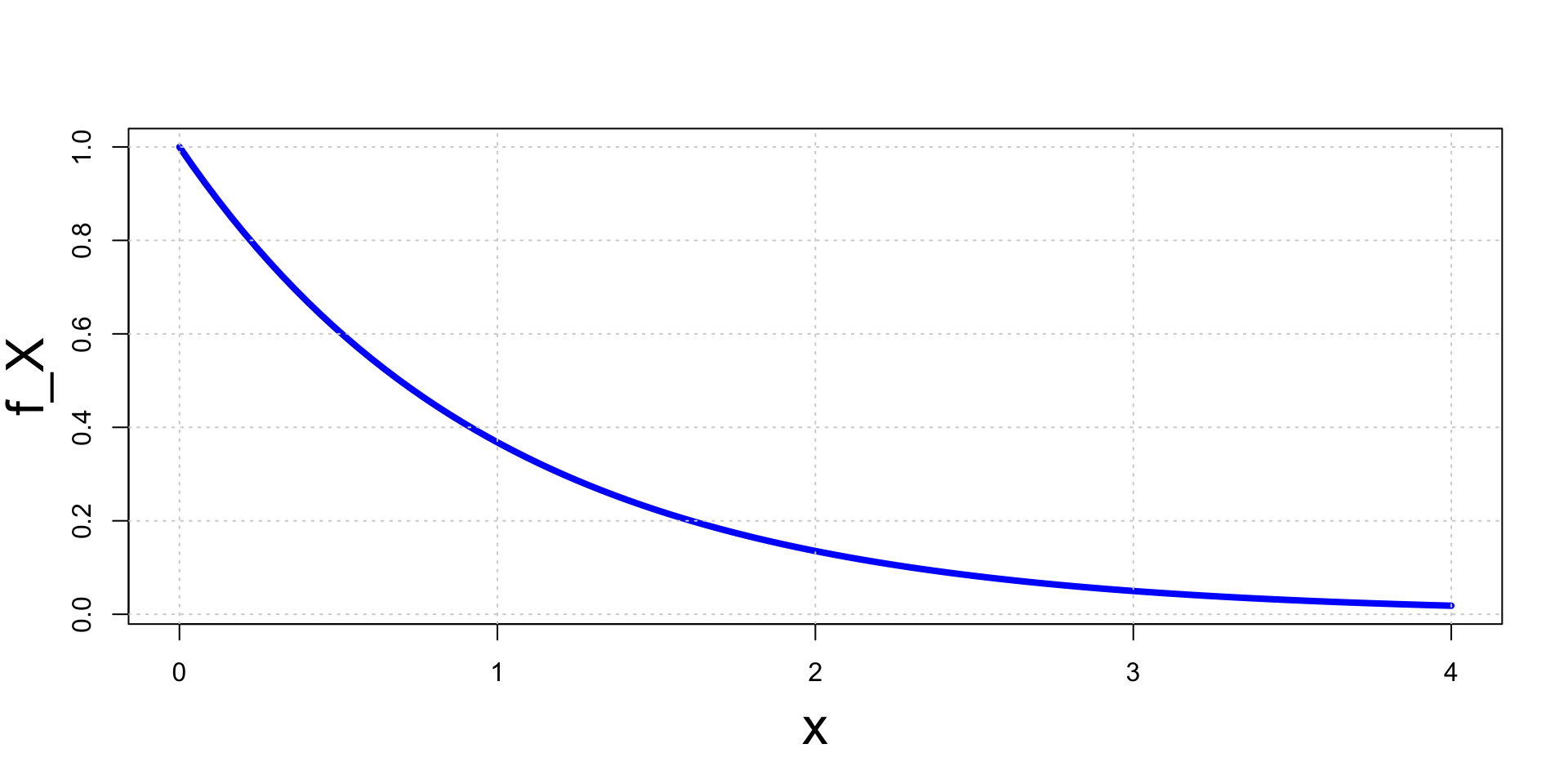
Example - Conditional distribution
- The marginal pdf of X has then exponential distribution f_{X}(x) = \begin{cases} e^{-x} & \text{ if } x > 0 \\ 0 & \text{ if } x \leq 0 \end{cases}
Example - Conditional distribution
- We now compute f(y|x), the conditional pdf of Y given X=x:
- Note that f_X(x)>0 for all x>0
- Hence assume fixed some x>0
- If y>x we have f_{X,Y}(x,y)=e^{-y}. Hence f(y|x) := \frac{f_{X,Y}(x,y)}{f_X(x)} = \frac{e^{-y}}{e^{-x}} = e^{-(y-x)}
- If y \leq x we have f_{X,Y}(x,y)=0. Hence f(y|x) := \frac{f_{X,Y}(x,y)}{f_X(x)} = \frac{0}{e^{-x}} = 0
Example - Conditional distribution
The conditional distribution Y|X is therefore exponential f(y|x) = \begin{cases} e^{-(y-x)} & \text{ if } y > x \\ 0 & \text{ if } y \leq x \end{cases}
The conditional expectation of Y given X=x is \begin{align*} {\rm I\kern-.3em E}[Y|x] & = \int_{-\infty}^\infty y f(y|x) \, dy = \int_{x}^\infty y e^{-(y-x)} \, dy \\ & = -(y+1) e^{-(y-x)} \bigg|_{x}^\infty = x + 1 \end{align*} where we integrated by parts
Example - Conditional distribution
Therefore conditional expectation of Y given X=x is {\rm I\kern-.3em E}[Y|x] = x + 1
This can also be interpreted as the random variable {\rm I\kern-.3em E}[Y|X] = X + 1
Example - Conditional distribution
The conditional second moment of Y given X=x is \begin{align*} {\rm I\kern-.3em E}[Y^2|x] & = \int_{-\infty}^\infty y^2 f(y|x) \, dy = \int_{x}^\infty y^2 e^{-(y-x)} \, dy \\ & = (y^2+2y+2) e^{-(y-x)} \bigg|_{x}^\infty = x^2 + 2x + 2 \end{align*} where we integrated by parts
The conditional variance of Y given X=x is {\rm Var}[Y|x] = {\rm I\kern-.3em E}[Y^2|x] - {\rm I\kern-.3em E}[Y|x]^2 = x^2 + 2x + 2 - (x+1)^2 = 1
This can also be interpreted as the random variable {\rm Var}[Y|X] = 1
Conditional Expectation
A useful formula
Theorem
(X,Y) random vector. Then
{\rm I\kern-.3em E}[X] = {\rm I\kern-.3em E}[ {\rm I\kern-.3em E}[X|Y] ]
Note: The above formula contains abuse of notation – {\rm I\kern-.3em E} has 3 meanings
- First {\rm I\kern-.3em E} is with respect to the marginal of X
- Second {\rm I\kern-.3em E} is with respect to the marginal of Y
- Third {\rm I\kern-.3em E} is with respect to the conditional distribution X|Y
Conditional Expectation
Proof of Theorem
Suppose (X,Y) is continuous
Recall that {\rm I\kern-.3em E}[X|Y] denotes the random variable g(Y) with g(y):= {\rm I\kern-.3em E}[X|y] := \int_{\mathbb{R}} xf(x|y) \, dx
Also recall that by definition f_{X,Y}(x,y)= f(x|y)f_Y(y)
Conditional Expectation
Proof of Theorem
Therefore \begin{align*} {\rm I\kern-.3em E}[{\rm I\kern-.3em E}[X|Y]] & = {\rm I\kern-.3em E}[g(Y)] = \int_{\mathbb{R}} g(y) f_Y(y) \, dy \\ & = \int_{\mathbb{R}} \left( \int_{\mathbb{R}} xf(x|y) \, dx \right) f_Y(y)\, dy = \int_{\mathbb{R}^2} x f(x|y) f_Y(y) \, dx dy \\ & = \int_{\mathbb{R}^2} x f_{X,Y}(x,y) \, dx dy = \int_{\mathbb{R}} x \left( \int_{\mathbb{R}} f_{X,Y}(x,y)\, dy \right) \, dx \\ & = \int_{\mathbb{R}} x f_{X}(x) \, dx = {\rm I\kern-.3em E}[X] \end{align*}
If (X,Y) is discrete the thesis follows by replacing intergrals with series
Conditional Expectation
Example - Application of the formula
Consider again the continuous random vector (X,Y) with joint pdf f_{X,Y}(x,y) := e^{-y} \,\, \text{ if } \,\, 0 < x < y \,, \quad f_{X,Y}(x,y) :=0 \,\, \text{ otherwise}
We have proven that {\rm I\kern-.3em E}[Y|X] = X + 1
We have also shown that f_X is exponential f_{X}(x) = \begin{cases} e^{-x} & \text{ if } x > 0 \\ 0 & \text{ if } x \leq 0 \end{cases}
Conditional Expectation
Example - Application of the formula
From the knowledge of f_X we can compute {\rm I\kern-.3em E}[X] {\rm I\kern-.3em E}[X] = \int_0^\infty x e^{-x} \, dx = -(x+1)e^{-x} \bigg|_{x=0}^{x=\infty} = 1
Using the Theorem we can compute {\rm I\kern-.3em E}[Y] without computing f_Y: \begin{align*} {\rm I\kern-.3em E}[Y] & = {\rm I\kern-.3em E}[ {\rm I\kern-.3em E}[Y|X] ] \\ & = {\rm I\kern-.3em E}[X + 1] \\ & = {\rm I\kern-.3em E}[X] + 1 \\ & = 1 + 1 = 2 \end{align*}
Part 3:
Independence
Independence of random variables
Intuition
In previous example: the conditional distribution of Y given X=x was f(y|x) = \begin{cases} e^{-(y-x)} & \text{ if } y > x \\ 0 & \text{ if } y \leq x \end{cases}
In particular f(y|x) depends on x
This means that knowledge of X gives information on Y
When X does not give any information on Y we say that X and Y are independent
Independence of random variables
Formal definition
Definition
(X,Y) random vector with joint pdf or pmf f_{X,Y} and marginal pdfs or pmfs f_X,f_Y. We say that X and Y are independent random variables if
f_{X,Y}(x,y) = f_X(x)f_Y(y) \,, \quad \forall \, (x,y) \in \mathbb{R}^2
Independence of random variables
Conditional distributions and probabilities
If X and Y are independent then X gives no information on Y (and vice-versa):
Conditional distribution: Y|X is same as Y f(y|x) = \frac{f_{X,Y}(x,y)}{f_X(x)} = \frac{f_X(x)f_Y(y)}{f_X(x)} = f_Y(y)
Conditional probabilities: From the above we also obtain \begin{align*} P(Y \in A | x) & = \sum_{y \in A} f(y|x) = \sum_{y \in A} f_Y(y) = P(Y \in A) & \, \text{ discrete rv} \\ P(Y \in A | x) & = \int_{y \in A} f(y|x) \, dy = \int_{y \in A} f_Y(y) \, dy = P(Y \in A) & \, \text{ continuous rv} \end{align*}
Independence of random variables
Characterization of independence - Densities
Theorem
(X,Y) random vector with joint pdf or pmf f_{X,Y}. They are equivalent:
- X and Y are independent random variables
- There exist functions g(x) and h(y) such that f_{X,Y}(x,y) = g(x)h(y) \,, \quad \forall \, (x,y) \in \mathbb{R}^2
Independence of random variables
Consequences of independence
Theorem
Suppose X and Y are independent random variables. Then
For any A,B \subset \mathbb{R} we have P(X \in A, Y \in B) = P(X \in A) P(Y \in B)
Suppose g(x) is a function of (only) x, h(y) is a function of (only) y. Then {\rm I\kern-.3em E}[g(X)h(Y)] = {\rm I\kern-.3em E}[g(X)]{\rm I\kern-.3em E}[h(Y)]
Independence of random variables
Proof of First Statement
Define the function p(x,y):=g(x)h(y). Then \begin{align*} {\rm I\kern-.3em E}[g(X)h(Y)] & = {\rm I\kern-.3em E}(p(X,Y)) = \int_{\mathbb{R}^2} p(x,y) f_{X,Y}(x,y) \, dxdy \\ & = \int_{\mathbb{R}^2} g(x)h(y) f_X(x) f_Y(y) \, dxdy \\ & = \left( \int_{-\infty}^\infty g(x) f_X(x) \, dx \right) \left( \int_{-\infty}^\infty h(y) f_Y(y) \, dy \right) \\ & = {\rm I\kern-.3em E}[g(X)] {\rm I\kern-.3em E}[h(Y)] \end{align*}
Proof in the discrete case is the same: replace intergrals with series
Independence of random variables
Proof of Second Statement
Define the product set A \times B :=\{ (x,y) \in \mathbb{R}^2 \colon x \in A , y \in B\}
Therefore we get \begin{align*} P(X \in A , Y \in B) & = \int_{A \times B} f_{X,Y}(x,y) \, dxdy \\ & = \int_{A \times B} f_X(x) f_Y(y) \, dxdy \\ & = \left(\int_{A} f_X(x) \, dx \right) \left(\int_{B} f_Y(y) \, dy \right) \\ & = P(X \in A) P(Y \in B) \end{align*}
Independence of random variables
Moment generating functions
Theorem
Suppose X and Y are independent random variables and denote by M_X and M_Y their moment generating functions. Then
M_{X + Y} (t) = M_X(t) M_Y(t)
Proof: Follows by previous Theorem \begin{align*} M_{X + Y} (t) & = {\rm I\kern-.3em E}[e^{t(X+Y)}] = {\rm I\kern-.3em E}[e^{tX}e^{tY}] \\ & = {\rm I\kern-.3em E}[e^{tX}] {\rm I\kern-.3em E}[e^{tY}] \\ & = M_X(t) M_Y(t) \end{align*}
Example
Sum of independent normals
Suppose X \sim N (\mu_1, \sigma_1^2) and Y \sim N (\mu_2, \sigma_2^2) are independent normal random variables
We have seen in Slide 119 in Lecture 1 that for normal distributions M_X(t) = \exp \left( \mu_1 t + \frac{t^2 \sigma_1^2}{2} \right) \,, \qquad M_Y(t) = \exp \left( \mu_2 t + \frac{t^2 \sigma_2^2}{2} \right)
Since X and Y are independent, from previous Theorem we get \begin{align*} M_{X+Y}(t) & = M_{X}(t) M_{Y}(t) = \exp \left( \mu_1 t + \frac{t^2 \sigma_1^2}{2} \right) \exp \left( \mu_2 t + \frac{t^2 \sigma_2^2}{2} \right) \\ & = \exp \left( (\mu_1 + \mu_2) t + \frac{t^2 (\sigma_1^2 + \sigma_2^2)}{2} \right) \end{align*}
Example
Sum of independent normals
Therefore Z := X + Y has moment generating function M_{Z}(t) = M_{X+Y}(t) = \exp \left( (\mu_1 + \mu_2) t + \frac{t^2 (\sigma_1^2 + \sigma_2^2)}{2} \right)
The above is the mgf of a normal distribution with \text{mean }\quad \mu_1 + \mu_2 \quad \text{ and variance} \quad \sigma_1^2 + \sigma_2^2
By the Theorem in Slide 132 of Lecture 1 we have Z \sim N(\mu_1 + \mu_2, \sigma_1^2 + \sigma_2^2)
Sum of independent normals is normal
Part 4:
Covariance and correlation
Relationship between Random Variables
Given two random variables X and Y we said that
X and Y are independent if f_{X,Y}(x,y) = f_X(x) g_Y(y)
In this case there is no relationship between X and Y
This is reflected in the conditional distributions: X|Y \sim X \qquad \qquad Y|X \sim Y
Relationship between Random Variables
If X and Y are not independent then there is a relationship between them
Question
How do we measure the strength of such dependence?
Answer: By introducing the notions of
- Covariance
- Correlation
Covariance
Definition
Notation: Given two rv X and Y we denote \begin{align*} & \mu_X := {\rm I\kern-.3em E}[X] \qquad & \mu_Y & := {\rm I\kern-.3em E}[Y] \\ & \sigma^2_X := {\rm Var}[X] \qquad & \sigma^2_Y & := {\rm Var}[Y] \end{align*}
Definition
The covariance of X and Y is the number
{\rm Cov}(X,Y) := {\rm I\kern-.3em E}[ (X - \mu_X) (Y - \mu_Y) ]
Covariance
Remark
The sign of {\rm Cov}(X,Y) gives information about the relationship between X and Y:
- If X is large, is Y likely to be small or large?
- If X is small, is Y likely to be small or large?
- Covariance encodes the above questions
Covariance
Remark
The sign of {\rm Cov}(X,Y) gives information about the relationship between X and Y
| X small: \, X<\mu_X | X large: \, X>\mu_X | |
|---|---|---|
| Y small: \, Y<\mu_Y | (X-\mu_X)(Y-\mu_Y)>0 | (X-\mu_X)(Y-\mu_Y)<0 |
| Y large: \, Y>\mu_Y | (X-\mu_X)(Y-\mu_Y)<0 | (X-\mu_X)(Y-\mu_Y)>0 |
| X small: \, X<\mu_X | X large: \, X>\mu_X | |
|---|---|---|
| Y small: \, Y<\mu_Y | {\rm Cov}(X,Y)>0 | {\rm Cov}(X,Y)<0 |
| Y large: \, Y>\mu_Y | {\rm Cov}(X,Y)<0 | {\rm Cov}(X,Y)>0 |
Covariance
Alternative Formula
Theorem
The covariance of X and Y can be computed via
{\rm Cov}(X,Y) = {\rm I\kern-.3em E}[XY] - {\rm I\kern-.3em E}[X]{\rm I\kern-.3em E}[Y]
Covariance
Proof of Theorem
Using linearity of {\rm I\kern-.3em E} and the fact that {\rm I\kern-.3em E}[c]=c for c \in \mathbb{R}: \begin{align*} {\rm Cov}(X,Y) : & = {\rm I\kern-.3em E}[ \,\, (X - {\rm I\kern-.3em E}[X]) (Y - {\rm I\kern-.3em E}[Y]) \,\, ] \\ & = {\rm I\kern-.3em E}\left[ \,\, XY - X {\rm I\kern-.3em E}[Y] - Y {\rm I\kern-.3em E}[X] + {\rm I\kern-.3em E}[X]{\rm I\kern-.3em E}[Y] \,\, \right] \\ & = {\rm I\kern-.3em E}[XY] - {\rm I\kern-.3em E}[ X {\rm I\kern-.3em E}[Y] ] - {\rm I\kern-.3em E}[ Y {\rm I\kern-.3em E}[X] ] + {\rm I\kern-.3em E}[{\rm I\kern-.3em E}[X] {\rm I\kern-.3em E}[Y]] \\ & = {\rm I\kern-.3em E}[XY] - {\rm I\kern-.3em E}[X] {\rm I\kern-.3em E}[Y] - {\rm I\kern-.3em E}[Y] {\rm I\kern-.3em E}[X] + {\rm I\kern-.3em E}[X] {\rm I\kern-.3em E}[Y] \\ & = {\rm I\kern-.3em E}[XY] - {\rm I\kern-.3em E}[X] {\rm I\kern-.3em E}[Y] \end{align*}
Correlation
Remark:
{\rm Cov}(X,Y) encodes only qualitative information about the relationship between X and Y
To obtain quantitative information we introduce the correlation
Definition
The correlation of X and Y is the number
\rho_{XY} := \frac{{\rm Cov}(X,Y)}{\sigma_X \sigma_Y}
Correlation
Correlation detects linear relationships between X and Y
Theorem
For any random variables X and Y we have
- - 1\leq \rho_{XY} \leq 1
- |\rho_{XY}|=1 if and only if there exist a,b \in \mathbb{R} such that Y = aX + b
- If \rho_{XY}=1 then a>0 \qquad \qquad \quad (positive linear correlation)
- If \rho_{XY}=-1 then a<0 \qquad \qquad (negative linear correlation)
Proof: Omitted, see page 172 of [1]
Correlation & Covariance
Independent random variables
Theorem
If X and Y are independent random variables then
{\rm Cov}(X,Y) = 0 \,, \qquad \rho_{XY}=0
Proof:
- If X and Y are independent then {\rm I\kern-.3em E}[XY]={\rm I\kern-.3em E}[X]{\rm I\kern-.3em E}[Y]
- Therefore {\rm Cov}(X,Y)= {\rm I\kern-.3em E}[XY]-{\rm I\kern-.3em E}[X]{\rm I\kern-.3em E}[Y] = 0
- Moreover \rho_{XY}=0 by definition
Formula for Variance
Variance is quadratic
Theorem
For any two random variables X and Y and a,b \in \mathbb{R}
{\rm Var}[aX + bY] = a^2 {\rm Var}[X] + b^2 {\rm Var}[Y] + 2 {\rm Cov}(X,Y)
If X and Y are independent then
{\rm Var}[aX + bY] = a^2 {\rm Var}[X] + b^2 {\rm Var}[Y]
Proof: Exercise
Part 5:
Multivariate random vectors
Multivariate Random Vectors
Recall
- A Random vector is a function \mathbf{X}\colon \Omega \to \mathbb{R}^n
- \mathbf{X} is a multivariate random vector if n \geq 3
- We denote the components of \mathbf{X} by \mathbf{X}= (X_1,\ldots,X_n) \,, \qquad X_i \colon \Omega \to \mathbb{R}
- We denote the components of a point \mathbf{x}\in \mathbb{R}^n by \mathbf{x}= (x_1,\ldots,x_n)
Discrete and Continuous Multivariate Random Vectors
Everything we defined for bivariate vectors extends to multivariate vectors
Definition
The random vector \mathbf{X}\colon \Omega \to \mathbb{R}^n is:
- continuous if components X_is are continuous
- discrete if components X_i are discrete
Joint pmf
Definition
The joint pmf of a continuous random vector \mathbf{X} is f_{\mathbf{X}} \colon \mathbb{R}^n \to \mathbb{R} defined by
f_{\mathbf{X}} (\mathbf{x}) = f_{\mathbf{X}}(x_1,\ldots,x_n) := P(X_1 = x_1 , \ldots , X_n = x_n ) \,, \qquad \forall \, \mathbf{x}\in \mathbb{R}^n
Note: For all A \subset \mathbb{R}^n it holds P(\mathbf{X}\in A) = \sum_{\mathbf{x}\in A} f_{\mathbf{X}}(\mathbf{x})
Joint pdf
Definition
The joint pdf of a continuous random vector \mathbf{X} is a function f_{\mathbf{X}} \colon \mathbb{R}^n \to \mathbb{R} such that
P (\mathbf{X}\in A) := \int_A f_{\mathbf{X}}(x_1 ,\ldots, x_n) \, dx_1 \ldots dx_n = \int_{A} f_{\mathbf{X}}(\mathbf{x}) \, d\mathbf{x}\,, \quad \forall \, A \subset \mathbb{R}^n
Note: \int_A denotes an n-fold intergral over all points \mathbf{x}\in A
Expected Value
Definition
\mathbf{X}\colon \Omega \to \mathbb{R}^n random vector and g \colon \mathbb{R}^n \to \mathbb{R} function. The expected value of the random variable g(X) is \begin{align*}
{\rm I\kern-.3em E}[g(\mathbf{X})] & := \sum_{x \in \mathbb{R}^n} g(\mathbf{x}) f_{\mathbf{X}} (\mathbf{x}) \qquad & (\mathbf{X}\text{ discrete}) \\
{\rm I\kern-.3em E}[g(\mathbf{X})] & := \int_{\mathbb{R}^n} g(\mathbf{x}) f_{\mathbf{X}} (\mathbf{x}) \, d\mathbf{x}\qquad & \qquad (\mathbf{X}\text{ continuous})
\end{align*}
Marginal distributions
Marginal pmf or pdf of any subset of the coordinates (X_1,\ldots,X_n) can be computed by integrating or summing the remaining coordinates
To ease notations, we only define maginals wrt the first k coordinates
Definition
The marginal pmf or marginal pdf of the random vector \mathbf{X} with respect to the first k coordinates is the function f \colon \mathbb{R}^k \to \mathbb{R} defined by \begin{align*}
f(x_1,\ldots,x_k) & := \sum_{ (x_{k+1}, \ldots, x_n) \in \mathbb{R}^{n-k} }
f_{\mathbf{X}} (x_1 , \ldots , x_n) \quad & (\mathbf{X}\text{ discrete}) \\
f(x_1,\ldots,x_k) & := \int_{\mathbb{R}^{n-k}}f_{\mathbf{X}} (x_1 , \ldots, x_n ) \, dx_{k+1} \ldots dx_{n} \quad & \quad (\mathbf{X}\text{ continuous})
\end{align*}
Marginal distributions
- We use a special notation for marginal pmf or pdf wrt a single coordinate
Definition
The marginal pmf or marginal pdf of the random vector \mathbf{X} with respect to the i-th coordinate is the function f_{X_i} \colon \mathbb{R}\to \mathbb{R} defined by \begin{align*}
f_{X_i}(x_i) & := \sum_{ \tilde{x} \in \mathbb{R}^{n-1} }
f_{\mathbf{X}} (x_1, \ldots, x_n) \quad & (\mathbf{X}\text{ discrete}) \\
f_{X_i}(x_i) & := \int_{\mathbb{R}^{n-1}}f_{\mathbf{X}} (x_1, \ldots, x_n) \, d\tilde{x} \quad & \quad (\mathbf{X}\text{ continuous})
\end{align*} where \tilde{x} \in \mathbb{R}^{n-1} denotes the vector \mathbf{x} with i-th component removed
\tilde{x} := (x_1, \ldots, x_{i-1}, x_{i+1},\ldots, x_n)
Conditional distributions
We now define conditional distributions given the first k coordinates
Definition
Let \mathbf{X} be a random vector and suppose that the marginal pmf or pdf wrt the first k coordinates satisfies
f(x_1,\ldots,x_k) > 0 \,, \quad \forall \, (x_1,\ldots,x_k ) \in \mathbb{R}^k
The conditional pmf or pdf of (X_{k+1},\ldots,X_n) given X_1 = x_1, \ldots , X_k = x_k is the function of (x_{k+1},\ldots,x_{n}) defined by
f(x_{k+1},\ldots,x_n | x_1 , \ldots , x_k) := \frac{f_{\mathbf{X}}(x_1,\ldots,x_n)}{f(x_1,\ldots,x_k)}
Conditional distributions
Similarly, we can define the conditional distribution given the i-th coordinate
Definition
Let \mathbf{X} be a random vector and suppose that for a given x_i \in \mathbb{R}
f_{X_i}(x_i) > 0
The conditional pmf or pdf of \tilde{X} given X_i = x_i is the function of \tilde{x} defined by
f(\tilde{x} | x_i ) := \frac{f_{\mathbf{X}}(x_1,\ldots,x_n)}{f_{X_i}(x_i)}
where we denote
\tilde{X} := (X_1, \ldots, X_{i-1}, X_{i+1},\ldots, X_n) \,, \quad
\tilde{x} := (x_1, \ldots, x_{i-1}, x_{i+1},\ldots, x_n)
Independence
Definition
\mathbf{X}=(X_1,\ldots,X_n) random vector with joint pmf or pdf f_{\mathbf{X}} and marginals f_{X_i}. We say that the random variables X_1,\ldots,X_n are mutually independent if
f_{\mathbf{X}}(x_1,\ldots,x_n) = f_{X_1}(x_1) \cdot \ldots \cdot f_{X_n}(x_n) = \prod_{i=1}^n f_{X_i}(x_i)
Proposition
If X_1,\ldots,X_n are mutually independent then for all A_i \subset \mathbb{R}
P(X_1 \in A_1 , \ldots , X_n \in A_n) = \prod_{i=1}^n P(X_i \in A_i)
Independence
Characterization result
Theorem
\mathbf{X}=(X_1,\ldots,X_n) random vector with joint pmf or pdf f_{\mathbf{X}}. They are equivalent:
- The random variables X_1,\ldots,X_n are mutually independent
- There exist functions g_i(x_i) such that f_{\mathbf{X}}(x_1,\ldots,x_n) = \prod_{i=1}^n g_{i}(x_i)
Independence
Expectation of product
Theorem
X_1,\ldots,X_n be mutually independent random variables and g_i(x_i) functions. Then
{\rm I\kern-.3em E}[ g_1(X_1) \cdot \ldots \cdot g_n(X_n) ] = \prod_{i=1}^n {\rm I\kern-.3em E}[g_i(X_i)]
Independence
A very useful theorem
Theorem
X_1,\ldots,X_n be mutually independent random variables and g_i(x_i) function only of x_i. Then the random variables
g_1(X_1) \,, \ldots \,, g_n(X_n)
are mutually independent
Proof: Omitted. See [1] page 184
Example: X_1,\ldots,X_n \, independent \,\, \implies \,\, X_1^2, \ldots, X_n^2 \, independent
Independence
MGF of sum
Theorem
X_1,\ldots,X_n be mutually independent random variables with mgfs M_{X_1}(t),\ldots, M_{X_n}(t). Define the random variable
Z := X_1 + \ldots + X_n
The mgf of Z satisfies
M_Z(t) = \prod_{i=1}^n M_{X_i}(t)
Sum of independent Normals
Theorem
Let X_1,\ldots,X_n be mutually independent random variables with normal distribution X_i \sim N (\mu_i,\sigma_i^2). Define
Z := X_1 + \ldots + X_n
and
\mu :=\mu_1 + \ldots + \mu_n \,, \quad \sigma^2 := \sigma_1^2 + \ldots + \sigma_n^2
Then Z is normally distributed with
Z \sim N(\mu,\sigma^2)
Sum of independent Normals
Proof of Theorem
We have seen in Slide 119 in Lecture 1 that if X_i \sim N(\mu_i,\sigma_i^2) then M_{X_i}(t) = \exp \left( \mu_i t + \frac{t^2 \sigma_i^2}{2} \right)
Since X_1,\ldots,X_n are mutually independent, from previous Theorem we get \begin{align*} M_{Z}(t) & = \prod_{i=1}^n M_{X_i}(t) = \prod_{i=1}^n \exp \left( \mu_i t + \frac{t^2 \sigma_i^2}{2} \right) \\ & = \exp \left( (\mu_1 + \ldots + \mu_n) t + \frac{t^2 (\sigma_1^2 + \ldots +\sigma_n^2)}{2} \right) \\ & = \exp \left( \mu t + \frac{t^2 \sigma^2 }{2} \right) \end{align*}
Sum of independent Normals
Proof of Theorem
Therefore Z has moment generating function M_{Z}(t) = \exp \left( \mu t + \frac{t^2 \sigma^2 }{2} \right)
The above is the mgf of a normal distribution with \text{mean }\quad \mu \quad \text{ and variance} \quad \sigma^2
Since mgfs characterize distributions (see Theorem in Slide 132 of Lecture 1), we conclude Z \sim N(\mu, \sigma^2 )
Sum of independent Gammas
Theorem
Let X_1,\ldots,X_n be mutually independent random variables with Gamma distribution X_i \sim \Gamma (\alpha_i,\beta). Define
Z := X_1 + \ldots + X_n
and
\alpha :=\alpha_1 + \ldots + \alpha_n
Then Z has Gamma distribution
Z \sim \Gamma(\alpha,\beta)
Sum of independent Gammas
Proof of Theorem
We have seen in Slide 126 in Lecture 1 that if X_i \sim \Gamma(\alpha_i,\beta) then M_{X_i}(t) = \frac{\beta^{\alpha_i}}{(\beta-t)^{\alpha_i}}
Since X_1,\ldots,X_n are mutually independent we get \begin{align*} M_{Z}(t) & = \prod_{i=1}^n M_{X_i}(t) = \prod_{i=1}^n \frac{\beta^{\alpha_i}}{(\beta-t)^{\alpha_i}} \\ & = \frac{\beta^{(\alpha_1 + \ldots + \alpha_n)}}{(\beta-t)^{(\alpha_1 + \ldots + \alpha_n)}} \\ & = \frac{\beta^{\alpha}}{(\beta-t)^{\alpha}} \end{align*}
Sum of independent Gammas
Proof of Theorem
Therefore Z has moment generating function M_{Z}(t) = \frac{\beta^{\alpha}}{(\beta-t)^{\alpha}}
The above is the mgf of a Gamma distribution with \text{mean }\quad \alpha \quad \text{ and variance} \quad \beta
Since mgfs characterize distributions (see Theorem in Slide 132 of Lecture 1), we conclude Z \sim \Gamma(\alpha, \beta )
Expectation of sums
Expectation is linear
Theorem
For random variables X_1,\ldots,X_n and scalars a_1,\ldots,a_n we have
{\rm I\kern-.3em E}[a_1X_1 + \ldots + a_nX_n] = a_1 {\rm I\kern-.3em E}[X_1] + \ldots + a_n {\rm I\kern-.3em E}[X_n]
Variance of sums
Variance is quadratic
Theorem
For random variables X_1,\ldots,X_n and scalars a_1,\ldots,a_n we have \begin{align*}
{\rm Var}[a_1X_1 + \ldots + a_nX_n] = a_1^2 {\rm Var}[X_1] & + \ldots + a^2_n {\rm Var}[X_n] \\
& + 2 \sum_{i \neq j} {\rm Cov}(X_i,X_j)
\end{align*} If X_1,\ldots,X_n are mutually independent then
{\rm Var}[a_1X_1 + \ldots + a_nX_n] = a_1^2 {\rm Var}[X_1] + \ldots + a^2_n {\rm Var}[X_n]
References
[1]
Casella, George, Berger, Roger L., Statistical inference, second edition, Brooks/Cole, 2002.