Statistical Models

Appendix

Dr. Silvio Fanzon

S.Fanzon@hull.ac.uk

University of Hull

Dr. John Fry

J.M.Fry@hull.ac.uk

University of Hull

Appendix:
More on R

Outline of Appendix

1. Functions in R
2. More on Vectors
3. Lists
4. Data Frames
5. Data Entry
6. R Style Guide

Part 1:
Functions in R

Expressions and objects

• Basic way to interact with R is through expression evaluation:
  • You enter an epression
  • The system evaluates it and prints the result
• Expressions work on objects
• Object: anything that can be assigned to a variable
• Objects encountered so far are:
  • Scalars
  • Vectors

Functions and arguments

• Functions are a class of objects

• Format of a function is name followed by parentheses containing arguments

• Functions take arguments and return a result

• We already encountered several built in functions:

  • plot(x, y)
  • lines(x, y)
  • seq(x)
  • print("Stats is great!")
  • cat("R is great!")
  • mean(x)
  • sin(x)

Functions and arguments

• Functions have actual arguments and formal arguments
• Example:
  • plot(x, y) has formal arguments two vectors x and y
  • plot(height, weight) has actual arguments height and weight
• When you write plot(height, weight) the arguments are matched:
  • height corresponds to x-variable
  • weight corresponds to y-variable
  • This is called positional matching

Functions and arguments

• If a function has a lot of arguments, positional matching is tedious

• For example plot() accepts the following (and more!) arguments

Argument	Description
x	x coordinate of points in the plot
y	y coordinate of points in the plot
type	Type of plot to be drawn
main	Title of the plot
xlab	Label of x axis
ylab	Label of y axis
pch	Shape of points

Functions and arguments

Issue with having too many arguments is the following:

• We might want to specify pch = 2
• But then we would have to match all the arguments preceding pch
  • x
  • y
  • type
  • xlab
  • ylab

Functions and arguments

• Thankfully we can use named actual arguments:
  • The name of a formal argument can be matched to an actual argument
  • This is independent of position
• For example we can specify pch = 2 by the call
  • plot(weight, height, pch = 2)
• In the above:
  • weight is implicitly matched to x
  • height is implicitly matched to y
  • pch is explicitly matched to 2
• Note that the following call would give same output
  • plot(x = weight, y = height, pch = 2)

Functions and arguments

• Named actual arguments override positional arguments
• Example: The following commands yield the same plot
  • plot(height, weight)
  • plot(x = height, y = weight)
  • plot(y = weight, x = height)

Functions and arguments

We have already seen another example of named actual arguments

• seq(from = 1, to = 11, by = 2)
• seq(1, 11, 2)
• These yield the same output. Why?
• Because in this case named actual arguments match positional arguments

Functions and arguments

If however we want to divide the interval [1, 11] in 5 equal parts:

• Have to use seq(1, 11, length.out = 6)

seq(1, 11, length.out = 6)

[1]  1  3  5  7  9 11

• The above is different from seq(1, 11, 6)

seq(1, 11, 6)

[1] 1 7

• They are different because:
  • The 3rd positional argument of seq() is by
  • Hence the command seq(1, 11, 6) assumes that by = 6

Functions and arguments

Warning

• You can call functions without specifying arguments
• However you have to use brackets ()
• Example:
  • getwd() – which outputs current working directory
  • ls() – which outputs names of objects currently in memory

Custom functions

• You can define your own functions in R
• Syntax for definining custom function my_function is below
• You can call your custom function by typing
  • my_function(arguments)

my_function <- function(first = "1st argument", 
                        ... ,
                        nth = "n-th argument") {
  
  # Code here: This is where you tell the function what to do

  return(object)      # Object to be returned  
}

Custom functions – Example

• The R function mean(x) computes the sample mean of vector x

• We want to define our own function to compute the mean

• Example: The mean of x could be computed via

  • sum(x) / length(x)

• We want to implement this code into the function my_mean(x)

  • my_mean takes vector x as argument
  • my_mean returns a scalar – the mean of x

# Definition of custom function my_mean(x)
my_mean <- function(vector = x) {
  
  mean_of_x <- sum(x) / length(x)
  
  return(mean_of_x)  
}

Custom functions – Example

• Let us use our function my_mean on an example

# Generate a random vector of 1000 entries from N(0,1)
x <- rnorm(1000)

# Compute mean of x with my_mean
xbar <- my_mean(x)

# Compute mean of x with built in function mean
xbar_check <- mean(x)
  
cat("Mean of x computed with my_mean is:", xbar)
cat("Mean of x computed with R mean is:", xbar_check)
cat("They coincide!")

Mean of x computed with my_mean is: 0.02337842

Mean of x computed with R mean is: 0.02337842

They coincide!

Part 2:
More on Vectors

More on vectors

• We have seen vectors of numbers
• Further type of vectors are:
  • Character vectors
  • Logical vectors

Character vectors

• A character vector is a vector of text strings
• Elements are specified and printed in quotes

x <- c("Red", "Green", "Blue")
print(x)

[1] "Red"   "Green" "Blue" 

• You can use single- or double-quote symbols to specify strings
• This is as long as the left quote is the same as the right quote

x <- c('Red', 'Green', 'Blue')
print(x)

[1] "Red"   "Green" "Blue" 

Character vectors

Print and cat produce different output on character vectors:

• print(x) prints all the strings in x separately
• cat(x) concatenates strings. There is no way to tell how many were there

x <- c("Red", "Green", "Blue")
print(x)
cat(x)

[1] "Red"   "Green" "Blue" 

Red Green Blue

y <- c("Red Green", "Blue")
print(y)
cat(y)

[1] "Red Green" "Blue"     

Red Green Blue

Logical vectors

• Logical vectors can take the values TRUE, FALSE or NA
• TRUE and FALSE can be abbreviated with T and F
• NA stands for not available

# Create logical vector
x <- c(T, T, F, T, NA)

# Print the logical vector
print(x)

[1]  TRUE  TRUE FALSE  TRUE    NA

Logical vectors

• Logical vectors are extremely useful to evaluate conditions

• Example:

  • given a numerical vector x
  • we want to count how many entries are above a value t

# Generate a vector containing sequence 1 to 8
x <- seq(from = 1 , to = 8, by = 1)

# Generate vector of flags for entries strictly above 5
y <- ( x > 5 )

cat("Vector x is: (", x, ")")
cat("Entries above 5 are: (", y, ")")

Vector x is: ( 1 2 3 4 5 6 7 8 )

Entries above 5 are: ( FALSE FALSE FALSE FALSE FALSE TRUE TRUE TRUE )

Logical vectors – Application

• Generate a vector of 1000 numbers from N(0,1)
• Count how many entries are above the mean 0
• Since there are many (1000) entries, we expect a result close to 500
  • This is because sample mean converges to true mean 0

Question: How to do this?

Hint: T/F are interpreted as 1/0 in arithmetic operations

T + T

[1] 2

T + F

[1] 1

F + F

[1] 0

F + T + 3

[1] 4

Logical vectors – Application

• The function sum(x) sums the entries of a vector x
• We can use sum(x) to count the number of T entries in a logical vector x

x <- rnorm(1000)       # Generates vector with 1000 normal entries

y <- (x > 0)           # Generates logical vector of entries above 0

above_zero <- sum(y)   # Counts entries above zero

cat("Number of entries which are above the average 0 is", above_zero)
cat("This is pretty close to 500!")

Number of entries which are above the average 0 is 472

This is pretty close to 500!

Missing values

• In practical data analysis, a data point is frequently unavailable
• Statistical software needs ways to deal with this
• R allows vectors to contain a special NA value - Not Available
• NA is carried through in computations: operations on NA yield NA as the result

2 * NA

[1] NA

NA + NA

[1] NA

T + NA

[1] NA

Indexing vectors

• Components of a vector can be retrieved by indexing

• vector[k] returns k-th component of vector

vector <- c("Cat", "Dog", "Mouse")

second_element <- vector[2]           # Access 2nd entry of vector

print(second_element)

[1] "Dog"

Replacing vector elements

To modify an element of a vector use the following:

• vector[k] <- value stores value in k-th component of vector

vector <- c("Cat", "Dog", "Mouse")

# We replace 2nd entry of vector with string "Horse"
vector[2] <- "Horse"

print(vector)

[1] "Cat"   "Horse" "Mouse"

Vector slicing

Returning multiple items of a vactor is known as slicing

• vector[c(k1, ..., kn)] returns components k1, ..., kn
• vector[k1:k2] returns components k1 to k2

vector <- c(11, 22, 33, 44, 55, 66, 77, 88, 99, 100)

# We store 1st, 3rd, 5th entries of vector in slice
slice <- vector[c(1, 3, 5)]   

print(slice)

[1] 11 33 55

Vector slicing

vector <- c(11, 22, 33, 44, 55, 66, 77, 88, 99, 100)

# We store 2nd to 7th entries of vector in slice
slice <- vector[2:7]

print(slice)

[1] 22 33 44 55 66 77

Deleting vector elements

• Elements of a vector x can be deleted by using
  • x[ -c(k1, ..., kn) ] which deletes entries k1, ..., kn

# Create a vector x
x <- c(11, 22, 33, 44, 55, 66, 77, 88, 99, 100)

# Print vector x
cat("Vector x is:", x)

# Delete 2nd, 3rd and 7th entries of x
x <- x[ -c(2, 3, 7) ]

# Print x again
cat("Vector x with 2nd, 3rd and 7th entries removed:", x)

Vector x is: 11 22 33 44 55 66 77 88 99 100

Vector x with 2nd, 3rd and 7th entries removed: 11 44 55 66 88 99 100

Logical Subsetting

• You can index or slice vectors by entering explicit indices
• You can also index vectors, or subset, by using logical flag vectors:
  • Element is extracted if corresponding entry in the flag vector is TRUE
  • Logical flag vectors should be the same length as vector to subset

Code: Suppose given a vector x

• Create a flag vector by using

  • flag <- condition(x)

• condition() is any function which returns T/F vector of same length as x

• Subset x by using

  • x[flag]

Logical Subsetting

Example

• The following code extracts negative components from a numeric vector
• This can be done by using
  • x[ x < 0 ]

# Create numeric vector x
x <- c(5, -2.3, 4, 4, 4, 6, 8, 10, 40221, -8)

# Get negative components from x and store them in neg_x
neg_x <- x[ x < 0 ]

cat("Vector x is:", x)
cat("Negative components of x are:", neg_x)

Vector x is: 5 -2.3 4 4 4 6 8 10 40221 -8

Negative components of x are: -2.3 -8

Logical Subsetting

Example

• The following code extracts components falling between a and b
• This can be done by using logical operator and &
  • x[ (x > a) & (x < b) ]

# Create numeric vector
x <- c(5, -2.3, 4, 4, 4, 6, 8, 10, 40221, -8)

# Get components between 0 and 100
range_x <- x[ (x > 0) & (x < 100) ]

cat("Vector x is:", x)
cat("Components of x between 0 and 100 are:", range_x)

Vector x is: 5 -2.3 4 4 4 6 8 10 40221 -8

Components of x between 0 and 100 are: 5 4 4 4 6 8 10

The function Which

• which() allows to convert a logical vector flag into a numeric index vector
  • which(flag) is vector of indices of flag which correspond to TRUE

# Create a logical flag vector
flag <- c(T, F, F, T, F)

# Indices for  flag which
true_flag <- which(flag)

cat("Flag vector is:", flag)
cat("Positions for which Flag is TRUE are:", true_flag)

Flag vector is: TRUE FALSE FALSE TRUE FALSE

Positions for which Flag is TRUE are: 1 4

The function Which – Application

which() can be used to delete certain entries from a vector x

• Create a flag vector by using

  • flag <- condition(x)

• condition() is any function which returns T/F vector of same length as x

• Delete entries flagged by condition using the code

  • x[ -which(flag) ]

The function Which – Application

Example

# Create numeric vector x
x <- c(5, -2.3, 4, 4, 4, 6, 8, 10, 40221, -8)

# Print x
cat("Vector x is:", x)

# Flag positive components of x
flag_pos_x <- (x > 0)

# Remove positive components from x
 x <- x[ -which(flag_pos_x) ]

# Print x again
cat("Vector x with positive components removed:", x)

Vector x is: 5 -2.3 4 4 4 6 8 10 40221 -8

Vector x with positive components removed: -2.3 -8

Functions that create vectors

The main functions to generate vectors are

• c() concatenate
• seq() sequence
• rep() replicate

We have already met c() and seq() but there are more details to discuss

Concatenate

Recall: c() generates a vector containing the input values

# Generate a vector of values 1, 2, 3, 4, 5
x <- c(1, 2, 3, 4, 5)

# Print the vector
print(x)

[1] 1 2 3 4 5

Concatenate

• c() can also concatenate vectors
• This was you can add entries to an existing vector

# Create 2 vectors
x <- c(1, 2, 3, 4, 5)
y <- c(6, 7, 8)

# Concatenate vectors x and y, and also add element 9
z <- c(x, y, 9)

# Print the resulting vector
print(z)

[1] 1 2 3 4 5 6 7 8 9

Concatenate

• You can assign names to vector elements

• This modifies the way the vector is printed

# We specify a vector with 3 named entries
x <- c(first = "Red", second = "Green", third = "Blue")

# Print the named vector
print(x)

  first  second   third 
  "Red" "Green"  "Blue" 

Concatenate

Given a named vector x

• Names can be extracted with names(x)
• Values can be extracted with unname(x)

# Create named vector
x <- c(first = "Red", second = "Green", third = "Blue")

# Access names of x via names(x)
names_x <- names(x)

# Access values of x via unname(x)
values_x <- unname(x)

cat("Names of x are:", names(x))
cat("Values of x are:", unname(x))

Names of x are: first second third

Values of x are: Red Green Blue

Concatenate

• All elements of a vector have the same type
• Concatenating vectors of different types leads to conversion

c(FALSE, 2)        # Converts FALSE to 0

[1] 0 2

c(pi, "stats")     # Converts pi to string 

[1] "3.14159265358979" "stats"           

c(TRUE, "stats")   # Converts TRUE to string

[1] "TRUE"  "stats"

Sequence

• Recall the syntax of seq is
  • seq(from =, to =, by =, length.out =)
• Omitting the third argument assumes that by = 1

# The following generates a vector of integers from 1 to 6
x <- seq(1, 6)

print(x)

[1] 1 2 3 4 5 6

Sequence

• seq(x1, x2) is equivalent to x1:x2
• Syntax x1:x2 is preferred to seq(x1, x2)

# Generate two vectors of integers from 1 to 6
x <- seq(1, 6)
y <- 1:6

cat("Vector x is:", x)
cat("Vector y is:", y)
cat("They are the same!")

Vector x is: 1 2 3 4 5 6

Vector y is: 1 2 3 4 5 6

They are the same!

Replicate

rep generates repeated values from a vector:

• x vector
• n integer
• rep(x, n) repeats n times the vector x

# Create a vector with 3 components
x <- c(2, 1, 3)

# Repeats 4 times the vector x
y <- rep(x, 4)

cat("Original vector is:", x)
cat("Original vector repeated 4 times:", y)

Original vector is: 2 1 3

Original vector repeated 4 times: 2 1 3 2 1 3 2 1 3 2 1 3

Replicate

The second argument of rep() can also be a vector:

• Given x and y vectors
• rep(x, y) repeats entries of x as many times as corresponding entries of y

x <- c(2, 1, 3)         # Vector to replicate
y <- c(1, 2, 3)         # Vector saying how to replicate 

z <- rep(x, y)          # 1st entry of x is replicated 1 time
                        # 2nd entry of x is replicated 2 times
                        # 3rd entry of x is replicated 3 times

cat("Original vector is:", x)
cat("Original vector repeated is:", z)

Original vector is: 2 1 3

Original vector repeated is: 2 1 1 3 3 3

Replicate

• rep() can be useful to create vectors of labels
• Example: Suppose we want to collect some numeric data on 3 Cats and 4 Dogs

x <- c("Cat", "Dog")     # Vector to replicate

y <- rep(x, c(3, 4))     # 1st entry of x is replicated 3 times
                         # 2nd entry of x is replicated 4 times

cat("Vector of labels is:", y)

Vector of labels is: Cat Cat Cat Dog Dog Dog Dog

Part 3:
Lists

Lists

• Vectors can contain only one data type (number, character, boolean)

• Lists are data structures that can contain any R object

• Lists can be created similarly to vectors, with the command list()

# List containing a number, a vector, and a string
my_list <- list(2, c(T,F,T,T), "hello")

# Print the list
print(my_list)

[[1]]
[1] 2

[[2]]
[1]  TRUE FALSE  TRUE  TRUE

[[3]]
[1] "hello"

Retrieving elements

Elements of a list can be retrieved by indexing

• my_list[[k]] returns k-th element of my_list

# Consider again the same list
my_list <- list(2, c(T,F,T,T), "hello")

# Access 2nd element of my_list and store it in variable
second_element <- my_list[[2]]

# In this case the variable second_element is a vector
print(second_element)

[1]  TRUE FALSE  TRUE  TRUE

List slicing

You can return multiple items of a list via slicing

• my_list[c(k1, ..., kn)] returns elements in positions k1, ..., kn
• my_list[k1:k2] returns elements k1 to k2

my_list <- list(2, c(T,F), "Cat", "Dog", pi, 42)

# We store 1st, 3rd, 5th entries of my_list in slice
slice <- my_list[c(1, 3, 5)]

print(slice)

[[1]]
[1] 2

[[2]]
[1] "Cat"

[[3]]
[1] 3.141593

List slicing

my_list <- list(2, c(T,F), "Cat", "Dog", pi, 42)

# We store 2nd to 4th entries of my_list in slice
slice <- my_list[2:4]

print(slice)

[[1]]
[1]  TRUE FALSE

[[2]]
[1] "Cat"

[[3]]
[1] "Dog"

Naming

• Components of a list can be named. Names can be assigned with
  • names(my_list) <- c("name_1", ..., "name_k")

# Create list with 3 elements
my_list <- list(2, c(T,F,T,T), "hello")

# Name each of the 3 elements
names(my_list) <- c("number", "TF_vector", "string")

# Print the named list: the list is printed along with element names 
print(my_list)

$number
[1] 2

$TF_vector
[1]  TRUE FALSE  TRUE  TRUE

$string
[1] "hello"

Accessing a name

• A component of my_list named my_name can be accessed with dollar operator
  • my_list$my_name

# Create list with 3 elements and name them
my_list <- list(2, c(T,F,T,T), "hello")
names(my_list) <- c("number", "TF_vector", "string")

# Access 2nd element using dollar operator and store it in variable
second_component <- my_list$TF_vector

# Print 2nd element
print(second_component)

[1]  TRUE FALSE  TRUE  TRUE

Part 4:
Data Frames

Data Frames

• Data Frames are the best way of presenting a data set in R:

  • Each variable has assigned a collection of recorded observations

• Data frames can contain any R object

• Data Frames are similar to Lists, with the difference that:

  • Members of a Data Frame must all be vectors of equal length

Constructing a Data Frame

• Data frames are constructed similarly to lists, using data.frame()

• Important: Elements of data frame must be vectors of the same length

• Example: We construct the Family Guy data frame. Variables are

  • person – Name of character
  • age – Age of character
  • sex – Sex of character

family <- data.frame(
  person = c("Peter", "Lois", "Meg", "Chris", "Stewie"),
  age = c(42, 40, 17, 14, 1),
  sex = c("M", "F" , "F", "M", "M")
)

Printing a Data Frame

• R prints data frames like matrices
• First row contains vector names

• First column contains row names
• Data are paired: e.g. Peter is 42 and Male

family <- data.frame(
  person = c("Peter", "Lois", "Meg", "Chris", "Stewie"),
  age = c(42, 40, 17, 14, 1),
  sex = c("M", "F" , "F", "M", "M")
)

print(family)

  person age sex
1  Peter  42   M
2   Lois  40   F
3    Meg  17   F
4  Chris  14   M
5 Stewie   1   M

Extracting data

• Think of a data frame as a matrix

• You can extract element in position (m,n) by using

  • my_data[m, n]

• Example: Peter is in 1st row. We can extract Peter’s name as follows

extracted <- family[1, 1]

print(extracted)

[1] "Peter"

Extracting data

To extract multiple elements on the same row or column type

• my_data[c(k1,...,kn), m] \quad or \quad my_data[k1:k2, m]
• my_data[n, c(k1,...,km)] \quad or \quad my_data[n, k1:k2]

Example: Meg is listed in 3rd row. We extract her age and sex

meg_data <- family[3, 2:3]

print(meg_data)

  age sex
3  17   F

Extracting data

To extract entire rows or columns type

• my_data[c(k1,...,kn), ] \quad or \quad my_data[k1:k2, ]
• my_data[, c(k1,...,km)] \quad or \quad my_data[, k1:k2]

peter_data <- family[1, ]      # Extracts first row - Peter
sex_age <- family[, c(3,2)]    # Extracts third and second columns:
                               # sex and age

print(peter_data)
print(sex_age)

  person age sex
1  Peter  42   M

  sex age
1   M  42
2   F  40
3   F  17
4   M  14
5   M   1

Extracting data

Use dollar operator to access data frame columns

• Suppose data set my_data contains a variable called my_variable
• my_data$my_variable accesses column my_variable
• my_data$my_variable is a vector

Example: To access age in the family data frame type

ages <- family$age        # Stores ages in a vector

cat("Ages of the Family Guy characters are", ages)
cat("Meg's age is", ages[3])

Ages of the Family Guy characters are 42 40 17 14 1

Meg's age is 17

Size of a data frame

The size of a data frame can be discovered using:

• nrow(my_data) \quad number of rows
• ncol(my_data) \quad number of columns
• dim(my_data) \quad \quad vector containing number of rows and columns

family_dim <- dim(family)    # Stores dimensions of family in a vector

cat("The Family Guy data frame has", family_dim[1], 
    "rows and", family_dim[2], "columns")

The Family Guy data frame has 5 rows and 3 columns

Adding Data

Adding data to an existing data frame my_data

• Add more records (adding to rows)
  • Create single row data frame new_record
  • new_record must match the structure of my_data
  • Add to my_data with my_data <- rbind(my_data, new_record)
• Add a set of observations for a new variable (adding to columns)
  • Create a vector new_variable
  • new_variable must have as many components as rows in my_data
  • Add to my_data with my_data <- cbind(my_data, new_variable)

Example: Add new record

• Consider the usual Family Guy data frame family
• Suppose we want to add data for Brian
• Create a new record: a single row data frame with columns
  • person, age, sex

new_record <- data.frame(
  person = "Brian",
  age = 7,
  sex = "M"
)

print(new_record)

  person age sex
1  Brian   7   M

Example: Add new record

• Now we add new_record to family

family <- rbind(family, new_record)

print(family)

  person age sex
1  Peter  42   M
2   Lois  40   F
3    Meg  17   F
4  Chris  14   M
5 Stewie   1   M
6  Brian   7   M

Example: Add new variable

• We want to add a new variable to the Family Guy data frame family
• This variable is called funny
• It records how funny each character is, with levels
  • Low, Med, High
• Create a vector funny with entries matching each character (including Brian)

funny <- c("High", "High", "Low", "Med", "High", "Med")

print(funny)

[1] "High" "High" "Low"  "Med"  "High" "Med" 

Example: Add new variable

• Add funny to the Family Guy data frame family

family <- cbind(family, funny)

print(family)

  person age sex funny
1  Peter  42   M  High
2   Lois  40   F  High
3    Meg  17   F   Low
4  Chris  14   M   Med
5 Stewie   1   M  High
6  Brian   7   M   Med

Adding a new variable: alternative way

Instead of using cbind we can add a new varibale using dollar operator:

• We want to add a variable called new_variable
• Create a vector v containing values for the new variable
• v must have as many components as rows in my_data
• Add to my_data with my_data$new_variable <- v

Adding a new variable: alternative way

Example:

• We add age expressed in months to the Family Guy data frame family
• Age in months can be computed by multiplying vector family$age by 12

v <- family$age * 12       # Computes vector of ages in months

family$age.months <- v     # Stores vector as new column in family

print(family)

  person age sex funny age.months
1  Peter  42   M  High        504
2   Lois  40   F  High        480
3    Meg  17   F   Low        204
4  Chris  14   M   Med        168
5 Stewie   1   M  High         12
6  Brian   7   M   Med         84

Logical Record Subsets

• We saw how to use logical flag vectors to subset vectors

• We can use logical flag vectors to subset data frames as well

• Suppose to have data frame my_data containing a variable my_variable

• Want to subset records in my_data for which my_variable satisfies a condition

• Use commands

  • flag <- condition(my_data$my_variable)
  • my_data[flag, ]

Logical Record Subsets

Example:

• Consider again the Family Guy data frame family
• We subset Male characters using flag family$sex == "M"

# Create flag vector for male Family Guy characters
flag <- (family$sex == "M")

# Subset data frame "family" and store in data frame "subset"
subset <- family[flag, ]

# Print subset
print(subset)

  person age sex funny age.months
1  Peter  42   M  High        504
4  Chris  14   M   Med        168
5 Stewie   1   M  High         12
6  Brian   7   M   Med         84

Part 5:
Data Entry

Reading data from files

• R has a many functions for reading characters from stored files

• We will see how to read Table-Format files

• Table-Formats are just tables stored in plain-text files

• Typical file estensions are:

  • .txt for plain-text files
  • .csv for comma-separated values

• Table-Formats can be read into R with the command

  • read.table()

Ta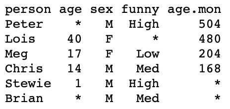ble-Formats

4 key features

1. Header:
   • If present, header should be the first line of the file
   • Header is used to provide names for each column of data
   • If a header is present, you need to tell this to R when importing
   • If not, R cannot tell if first line is a header or observed data values

Table-Formats

4 key features

2. Delimiter:
   • A character used to separate the entries in each line
   • Delimiter character cannot be used for anything else in the file
   • Delimiter tells R when a specific entry begins and ends
   • Default delimiter is whitespace

Table-Formats

4 key features

3. Missing value:
   • Character string used exclusively to denote a missing value
   • When reading the file, R will turn these entries into NA

Table-Formats

4 key features

4. Comments:
   • Table files can include comments
   • Comment lines start with \quad #
   • R ignores such comments

Table-Formats

Example

• Table-Format for Family Guy characters can be downloaded here family_guy.txt

• The text file looks like this

• Remarks:
  • Header is present
  • Delimiter is whitespace
  • Missing values denoted by *

read.table command

• Table-Formats can be read via read.table()
  • This reads a .txt or .csv file and outputs a data frame
• Options of read.table()
  • header = T/F – Tells R if a header is present
  • na.strings = "string" – Tells R that "string" means NA

Reading our first Table-Format file

To read family_guy.txt into R proceed as follows:

1. Download family_guy.txt and move file to Desktop

2. Open the R Console and change working directory to Desktop

# In MacOS type
setwd("~/Desktop")

# In Windows type
setwd("C:/Users/YourUsername/Desktop")

Reading our first Table-Format file

3. Read family_guy.txt into R and store it in data frame family with code

family = read.table(file = "family_guy.txt",
                    header = TRUE,
                    na.strings = "*"
                    )

4. Note that we are telling read.table() that
   • family_guy.txt has a header
   • Missing values are denoted by *

Reading our first Table-Format file

5. Print data frame family to screen

print(family)

  person age sex funny age.mon
1  Peter  NA   M  High     504
2   Lois  40   F  <NA>     480
3    Meg  17   F   Low     204
4  Chris  14   M   Med     168
5 Stewie   1   M  High      NA
6  Brian  NA   M   Med      NA

• For comparison this is the .txt file

Application: t-test

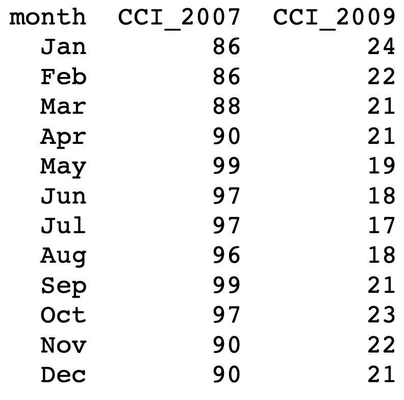
Example: Analysis of Consumer Confidence Index for 2008 crisis from Lecture 4

• We imported data into R using c()
• This is ok for small datasets
• Suppose the CCI data is stored in a .txt file instead

Goal: Perform t-test on CCI difference for mean difference \mu = 0

• By reading CCI data into R using read.table()
• By manipulating CCI data using data frames

Application: t-test

• The CCI dataset can be downloaded here 2008_crisis.txt

• The text file looks like this

Application: t-test

To perform the t-test on data 2008_crisis.txt we proceed as follows:

1. Download dataset 2008_crisis.txt and move file to Desktop

2. Open the R Console and change working directory to Desktop

# In MacOS type
setwd("~/Desktop")

# In Windows type
setwd("C:/Users/YourUsername/Desktop")

3. Read 2008_crisis.txt into R and store it in data frame scores with code

scores = read.table(file = "2008_crisis",
                    header = TRUE
                    )

Application: t-test

4. Store 2nd and 3rd columns of scores into 2 vectors

# CCI from 2007 is stored in 2nd column
score_2007 <- scores[, 2]

# CCI from 2009 is stored in 3nd column
score_2009 <- scores[, 3]

5. Now the t-test can be performed as done in Lecture 4

# Compute vector of differences
difference <- score_2007 - score_2009

# Perform t-test on difference with null hypothesis mu = 0
t.test(difference, mu = 0)

Application: t-test

6. We obtain the same result of Lecture 4
   • p-value is p < 0.05
   • Reject H_0: The mean difference is not 0
   • In details, the output of t.test is below

• For convenience you can download the full code 2008_crisis_code.R

    One Sample t-test

data:  difference
t = 38.144, df = 11, p-value = 4.861e-13
alternative hypothesis: true mean is not equal to 0
95 percent confidence interval:
 68.15960 76.50706
sample estimates:
mean of x 
 72.33333 

Part 6:
R Style Guide

R Style Guide

• Styling your code is optional
• However it is considered good manners to do so
• Good coding style makes code more readable
• Highly recommended, especially for assignments
• The next few slides on Style are based on these two posts:
  • Style Guide by Hadley Wickham (link)
  • Google’s R Style Guide (link)

File names

They should be meaningful and end in .R

# Good
football-models.R  
utility-functions.R
homework_1.R
homework1.R

# Bad
footballmodels.r # Hard to read
stuff.r          # What is inside this file?
code.r           # Same as above

Objects names

• Objects names shoulde be lowercase
• Use an underscore (_) to separate words within a name
• Variable names should be nouns, not verbs
• Come up with names that are concise and meaningful

# Good
day_one  # This will clearly store the value of first day
day_1    # Still clear


# Bad
first_day_of_the_month  # Too long
dayone                  # Hard to read
DayOne                  # Mix of upper and lower case
fdm                     # Hard to guess what this means

Functions names

• Name functions with BigCamelCase (link)
• This is to clearly distinguish functions from other objects
• Functions names should be verbs
• Come up with names that are concise and meaningful

# Good
DoNothing <- function() {
  return(invisible(NULL))
}

# Bad
donothing <- function() {
  return(invisible(NULL))
}

Object and functions names

If possible avoid using names of existing functions and variables

# Bad
T <- FALSE                  # T is reserved for the boolean TRUE
c <- 10                     # c denotes the concatenation operator
mean <- function(x) sum(x)  # mean already denotes a built in function

Assignment

Use <- and not = for assignment

# Good
x <- 5

# Bad
x = 5

Spacing

• Spacing is really something you should be careful about
• Place spaces around all infix operators (=, +, -, <-, etc.)
• Place spaces around = when calling a function
• Always put a space after a comma, never before (like in regular English)

# Good
average <- mean(feet / 12 + inches, na.rm = TRUE)

# Bad
average<-mean(feet/12+inches,na.rm=TRUE)

Spacing with Brackets

• Do not place spaces around code in parentheses or square brackets
• Unless there is a comma

# Good
if (condition) do(x)
diamonds[5, ]

# Bad
if ( condition ) do(x)  # No spaces around condition
x[1,]                   # Needs a space after the comma
x[1 ,]                  # Space goes after comma not before

Spacing - Exceptions

• Symbols :, :: and ::: do not need spacing

# Good
x <- 1:10

# Bad
x <- 1 : 10

• Place a space before left parentheses, except in a function call

#Good
if (condition) do(x)
plot(x, y)

# Bad
if(condition)do(x)    # (condition) needs spacing
plot (x, y)           # This does not need spacing

Extra Spacing

Extra spacing is ok if it improves alignment of = or <-

list(
  total = a + b + c, 
  mean  = (a + b + c) / n
)

Curly braces

• An opening curly brace should never go on its own line
• An opening curly brace should always be followed by a new line
• Always indent the code inside curly braces

# Good

if (y < 0 && debug) {
  message("Y is negative")
}

if (y == 0) {
  log(x)
} 

# Bad

if (y < 0 && debug)
message("Y is negative")


if (y == 0) 
{
  log(x)} 

Line length

• Limit code to 80 characters per line
• This fits comfortably on a printed page
• If you run out of room, encapsulate some of the work in separate function

Indentation

• When indenting your code, use two spaces
• Never use tabs or mix tabs and spaces
• Indentation should be used for functions, if, for, etc.

SumTwoNumbers <- function(x, y) {
  s = x + y
  return(s)
}

Indentation - Exception

If a function definition runs over multiple lines, indent the second line to where the definition starts

long_function_name <- function(a = "a long argument", 
                               b = "another argument",
                               c = "another long argument") {
  # As usual code is indented by two spaces.
}

Use explicit returns

• Functions can return objects
• R has an implicit return feature
• Do not rely on this feature, but explicitly mention return(object)

# Good
AddValues <- function(x, y) {
  return(x + y)                     # Function returns x+y
}

# Bad
AddValues <- function(x, y) {
  x + y                             # Function still returns x+y
}                                   # but it is not immediate to see it

Named arguments

• Often you can call a function without explicitly naming arguments:

  • plot(height, weight)
  • mean(weight)

• This might be fine for plot() or mean

• However for less common functions:

  • One might struggle to remember the meaning of arguments positions
  • It is therefore good practice to name arguments

# Good
seq(from = 1, to = 11, by = 1)

# Bad
seq(1, 11, 1)

Comments

• Most importantly: Comment your code
• Each line of a comment should begin with comment symbol # and a single space

# Here we sum two numbers  
x+y

• Use commented lines of - and = to break up code into easily readable chunks

# Load data ---------------------------

# Plot data ---------------------------