Statistical Models

Lecture 11

Dr. Silvio Fanzon

S.Fanzon@hull.ac.uk

University of Hull

Dr. John Fry

J.M.Fry@hull.ac.uk

University of Hull

Lecture 11:
Violation of regression
assumptions

Outline of Lecture 11

1. Regression modelling assumptions
2. Heteroscedasticity
3. Autocorrelation
4. Multicollinearity
5. Stepwise regression and overfitting
6. Dummy variable regression models

Part 1:
Regression assumptions

Regression modelling assumptions

In Lecture 9 we have introduced the general linear regression model

Y_i = \beta_1 z_{i1} + \beta_2 z_{i2} + \ldots + \beta_p z_{ip} + \varepsilon_i

• There are p predictor random variables

Z_1 \, , \,\, \ldots \, , \, Z_p

• Y_i is the conditional distribution

Y | Z_1 = z_{i1} \,, \,\, \ldots \,, \,\, Z_p = z_{ip}

• The errors \varepsilon_i are random variables

Regression assumptions on Y_i

1. Predictor is known: The values z_{i1}, \ldots, z_{ip} are known

2. Normality: The distribution of Y_i is normal

3. Linear mean: There are parameters \beta_1,\ldots,\beta_p such that {\rm I\kern-.3em E}[Y_i] = \beta_1 z_{i1} + \ldots + \beta_p z_{ip}

4. Homoscedasticity: There is a parameter \sigma^2 such that {\rm Var}[Y_i] = \sigma^2

5. Independence: rv Y_1 , \ldots , Y_n are independent and thus uncorrelated

{\rm Cor}(Y_i,Y_j) = 0 \qquad \forall \,\, i \neq j

Equivalent assumptions on \varepsilon_i

1. Predictor is known: The values z_{i1}, \ldots, z_{ip} are known

2. Normality: The distribution of \varepsilon_i is normal

3. Linear mean: The errors have zero mean {\rm I\kern-.3em E}[\varepsilon_i] = 0

4. Homoscedasticity: There is a parameter \sigma^2 such that {\rm Var}[\varepsilon_i] = \sigma^2

5. Independence: Errors \varepsilon_1 , \ldots , \varepsilon_n are independent and thus uncorrelated

{\rm Cor}(\varepsilon_i, \varepsilon_j) = 0 \qquad \forall \,\, i \neq j

Extra assumption on design matrix

6. The design matrix Z is such that

Z^T Z \, \text{ is invertible}

• Assumptions 1-6 allowed us to estimate the parameters

\beta = (\beta_1, \ldots, \beta_p)

• By maximizing the likelihood we obtained estimator

\hat \beta = (Z^T Z)^{-1} Z^T y

Violation of Assumptions

We consider 3 scenarios

1. Heteroscedasticity: The violation of Assumption 4 of homoscedasticity

{\rm Var}[\varepsilon_i] \neq {\rm Var}[\varepsilon_j] \qquad \text{ for some } \,\, i \neq j

2. Autocorrelation: The violation of Assumption 5 of no-correlation

{\rm Cor}( \varepsilon_i, \varepsilon_j ) \neq 0 \qquad \text{ for some } \,\, i \neq j

3. Multicollinearity: The violation of Assumption 6 of invertibilty of the matrix

Z^T Z

Part 2:
Heteroscedasticity

Heteroscedasticity

• The general linear regression model is

Y_i = \beta_1 z_{i1} + \beta_2 z_{i2} + \ldots + \beta_p z_{ip} + \varepsilon_i

• Consider Assumption 4
  • Homoscedasticity: There is a parameter \sigma^2 such that {\rm Var}[\varepsilon_i] = \sigma^2 \qquad \forall \,\, i
• Heteroscedasticity: The violation of Assumption 4

{\rm Var}[\varepsilon_i] \neq {\rm Var}[\varepsilon_j] \qquad \text{ for some } \,\, i \neq j

Why is homoscedasticity important?

• In Lecture 10 we presented a few methods to assess linear models

  • Coefficient R^2
  • t-tests for parameters significance
  • F-test for model selection

• The above methods rely heavily on homoscedasticity

Why is homoscedasticity important?

• For example the maximum likelihood estimation relied on the calculation \begin{align*} L & = \prod_{i=1}^n f_{Y_i} (y_i) = \prod_{i=1}^n \frac{1}{\sqrt{2\pi \sigma^2}} \exp \left( -\frac{(y_i - \hat y_i)^2}{2\sigma^2} \right) \\[15pts] & = \frac{1}{(2\pi \sigma^2)^{n/2}} \, \exp \left( -\frac{\sum_{i=1}^n(y_i- \hat y_i)^2}{2\sigma^2} \right) \\[15pts] & = \frac{1}{(2\pi \sigma^2)^{n/2}} \, \exp \left( -\frac{ \mathop{\mathrm{RSS}}}{2\sigma^2} \right) \end{align*}

• The calculation is only possible thanks to homoscedasticity

{\rm Var}[Y_i] = \sigma^2 \qquad \forall \,\, i

Why is homoscedasticity important?

• Suppose the calculation in previous slide holds

L = \frac{1}{(2\pi \sigma^2)^{n/2}} \, \exp \left( -\frac{ \mathop{\mathrm{RSS}}}{2\sigma^2} \right)

• Then maximizing the likelihood is equivalent to solving

\min_{\beta} \ \mathop{\mathrm{RSS}}

• The above has the closed form solution

\hat \beta = (Z^T Z)^{-1} Z^T y

Why is homoscedasticity important?

• Without homoscedasticity we would have

L \neq \frac{1}{(2\pi \sigma^2)^{n/2}} \, \exp \left( -\frac{ \mathop{\mathrm{RSS}}}{2\sigma^2} \right)

• Therefore \hat \beta would no longer maximize the likelihood!

• In this case \hat \beta would still be an unbiased estimator for \beta

{\rm I\kern-.3em E}[\hat \beta ] = \beta

Why is homoscedasticity important?

• However the quantity S^2 = \frac{ \mathop{\mathrm{RSS}}(\hat \beta) }{n-p} is not anymore unbiased estimator for the population variance \sigma^2 {\rm I\kern-.3em E}[S^2] \neq \sigma^2

• This is a problem because the estimated standard error for \beta_j involves S^2 \mathop{\mathrm{e.s.e.}}(\beta_j) = \xi_{jj}^{1/2} \, S

• Therefore \mathop{\mathrm{e.s.e.}} becomes unreliable

Why is homoscedasticity important?

• Then also t-statistic for significance of \beta_j becomes unreliable

• This is because the t-statistic depends on \mathop{\mathrm{e.s.e.}}

t = \frac{ \hat\beta_j - \beta_j }{ \mathop{\mathrm{e.s.e.}}}

• Without homoscedasticity the regression maths does not work!
  • t-tests for significance of \beta_j
  • confidence intervals for \beta_j
  • F-tests for model selection
  • They all break down and become unreliable!

Is heteroscedastcity a serious problem?

• Heteroscedasticity in linear regression is no longer a big problem

• This is thanks to 1980s research on robust standard errors (more info here)

• Moreover heteroscedasticity only becomes a problem when it is severe

How to detect Heteroscedasticity

• Heteroscedasticity is commonly present in real-world datasets
  • We should be able to detect it

• There are formal tests (see [1])
  • Goldfeldt-Quant test
  • White’s test for heteroscedasticity

How to detect Heteroscedasticity

• Alternative: graphical checks
  • Simpler and more robust
• They involve studying the model residuals

e_i := y_i - \hat y_i

• By definition e_i is sampled from \varepsilon_i

• We have heteroscedasticity if

{\rm Var}[\varepsilon_i] \neq {\rm Var}[\varepsilon_j] \, \quad \, \text{ for some } \, i \neq j

• Hence under heteroscedasticity the residuals e_i have different variance

Graphical checks

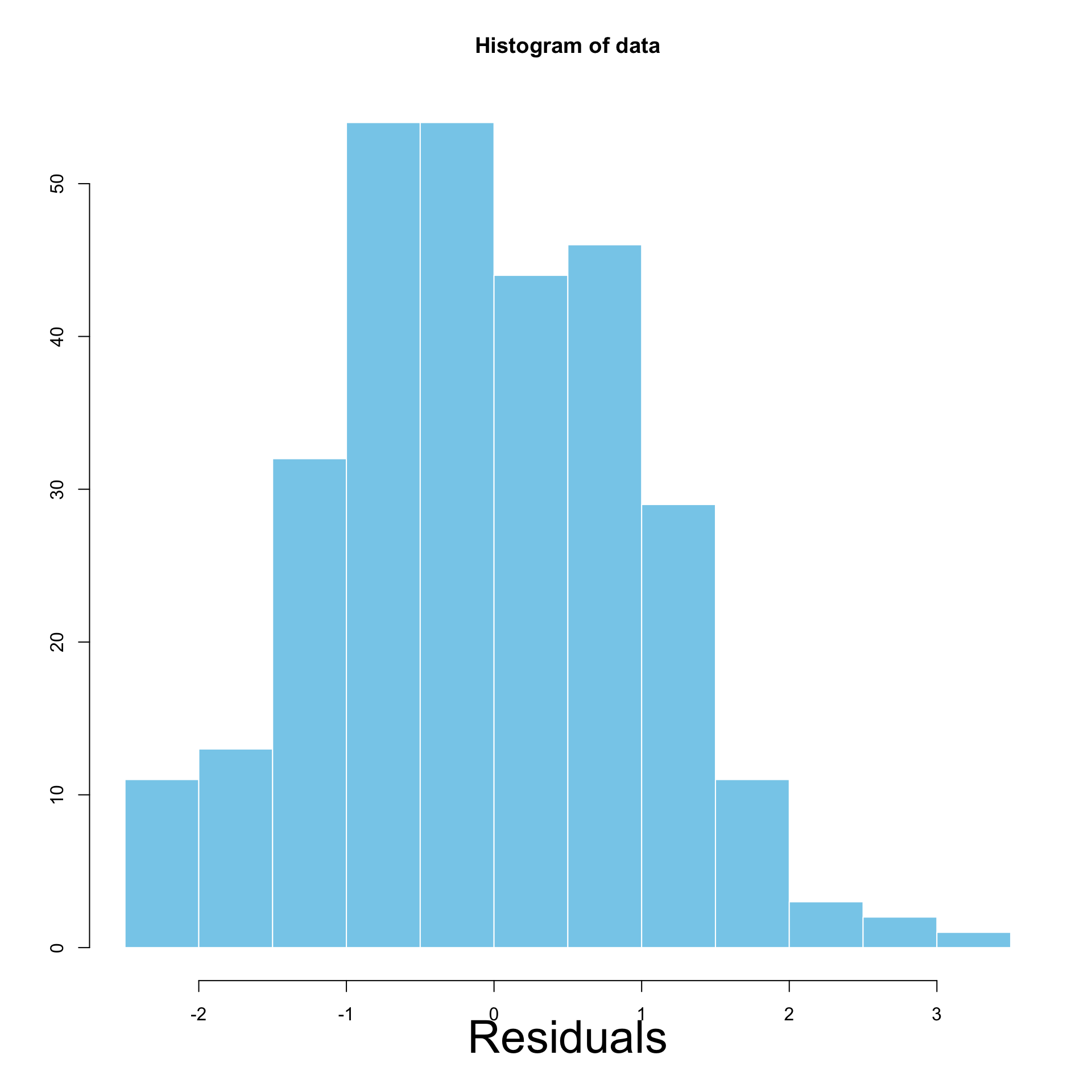
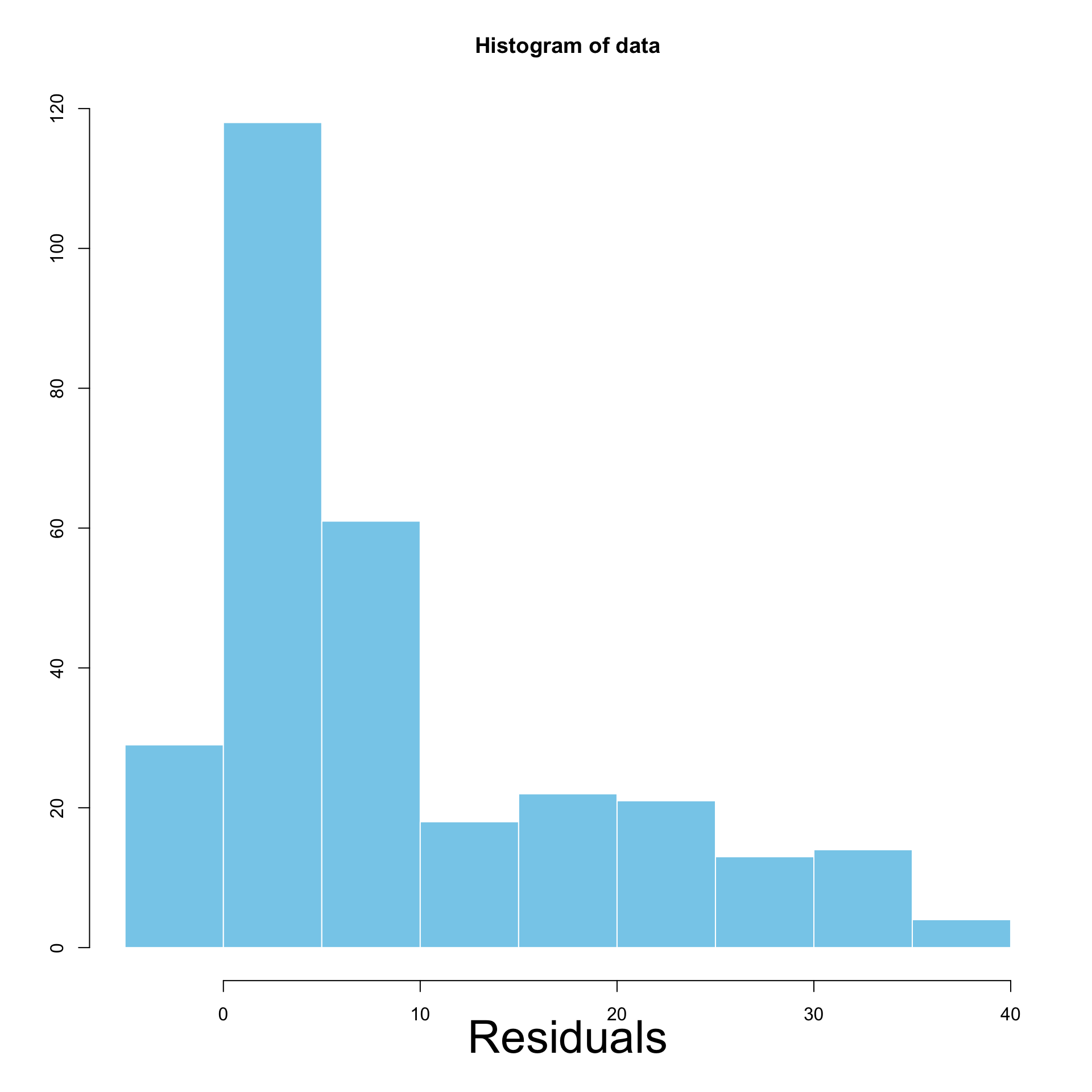
First method: Histogram of residuals

• Yes Heteroscedasticity:
  • Residuals have different variance
  • Histogram will display asymetric pattern
• No Heteroscedasticity:
  • Homoscedasticity assumption holds
  • Residuals have same variance
  • Histogram will look like normal distribution N(0,\sigma^2)

Interpretation of Histograms

Left: Homoscedastic \qquad\quad\quad Right: Heteroscedastic

Graphical checks

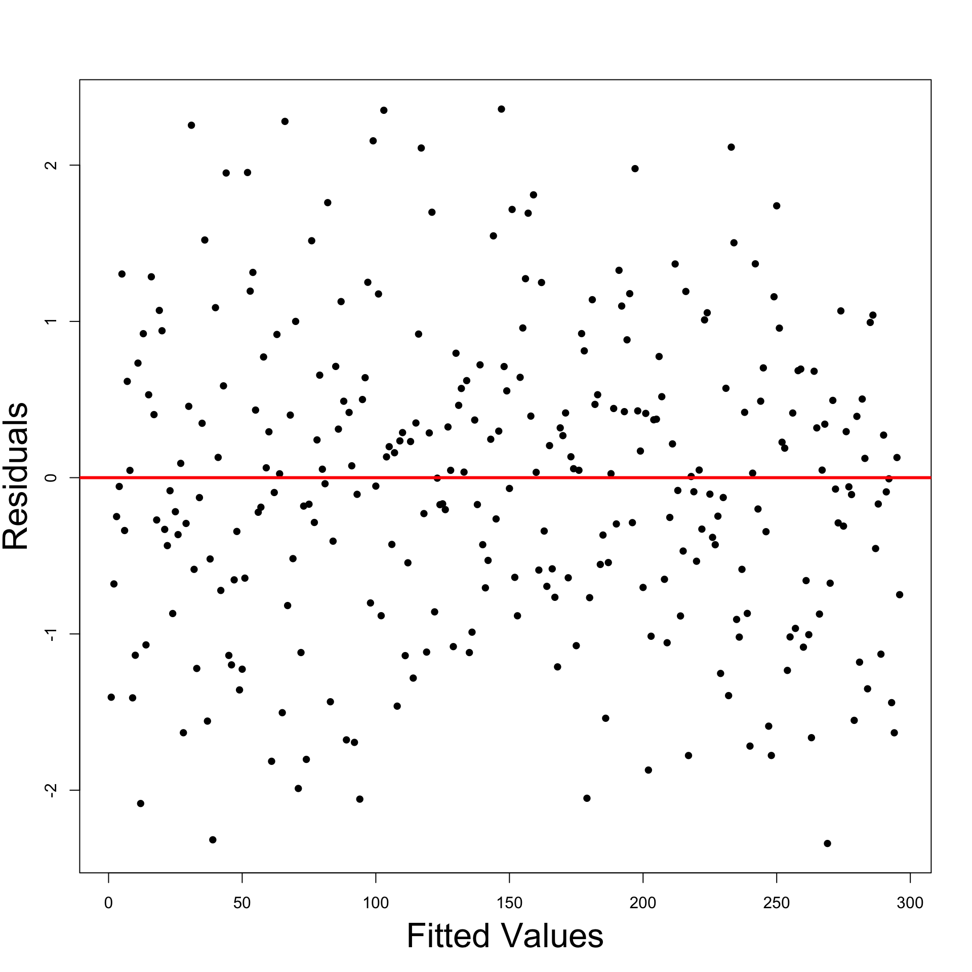
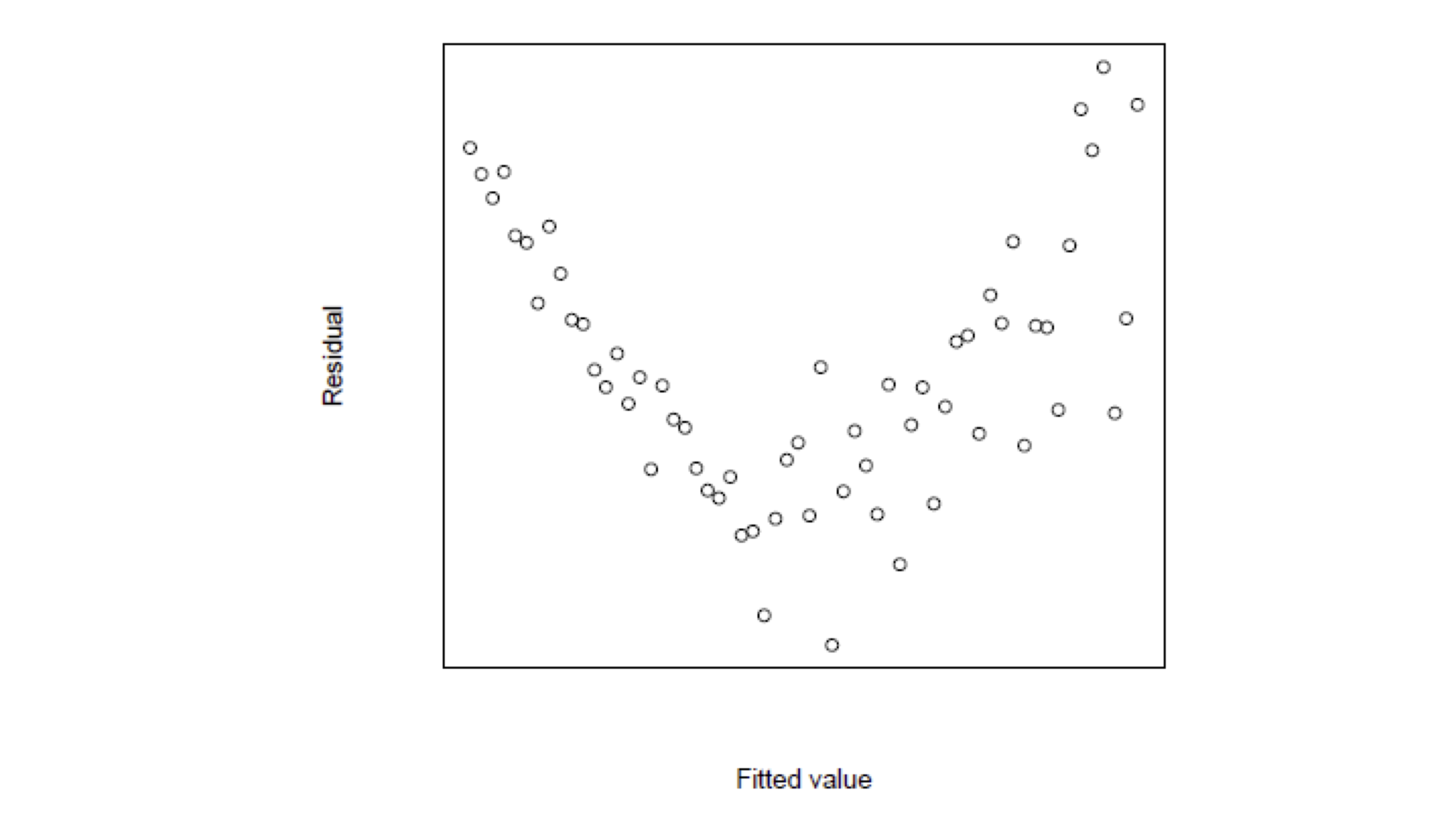
Second method: Residual graphs

• Residual graphs are plots of
  • Residuals against fitted values
  • Squared residuals against fitted values
• Important:
  • No Heteroscedasticity: Plots will look random
  • Yes Heteroscedasticity: Plots will show certain patterns
• Good reference is the book [2]

Interepretation of Residual Graphs

• No systematic pattern:
  • Suggests no heteroscedasticity
  • Corresponds to constant variance
  • Homoscedasticity assumption holds
• Residuals resemble sample N(0,\sigma^2)
  • About half residuals negative and half positive
  • Vertical spread is comparable

Interepretation of Residual Graphs

Patterns implying Heteroscedasticity

1. Funnelling out of residuals

2. Funnelling in of residuals

3. Linear residuals – Proportional to \hat y_i

4. Quadratic residuals – Proportional to \hat{y}^2_i

In these special cases we can transform the data to avoid heteroscedasticity

Funnelling out of residuals

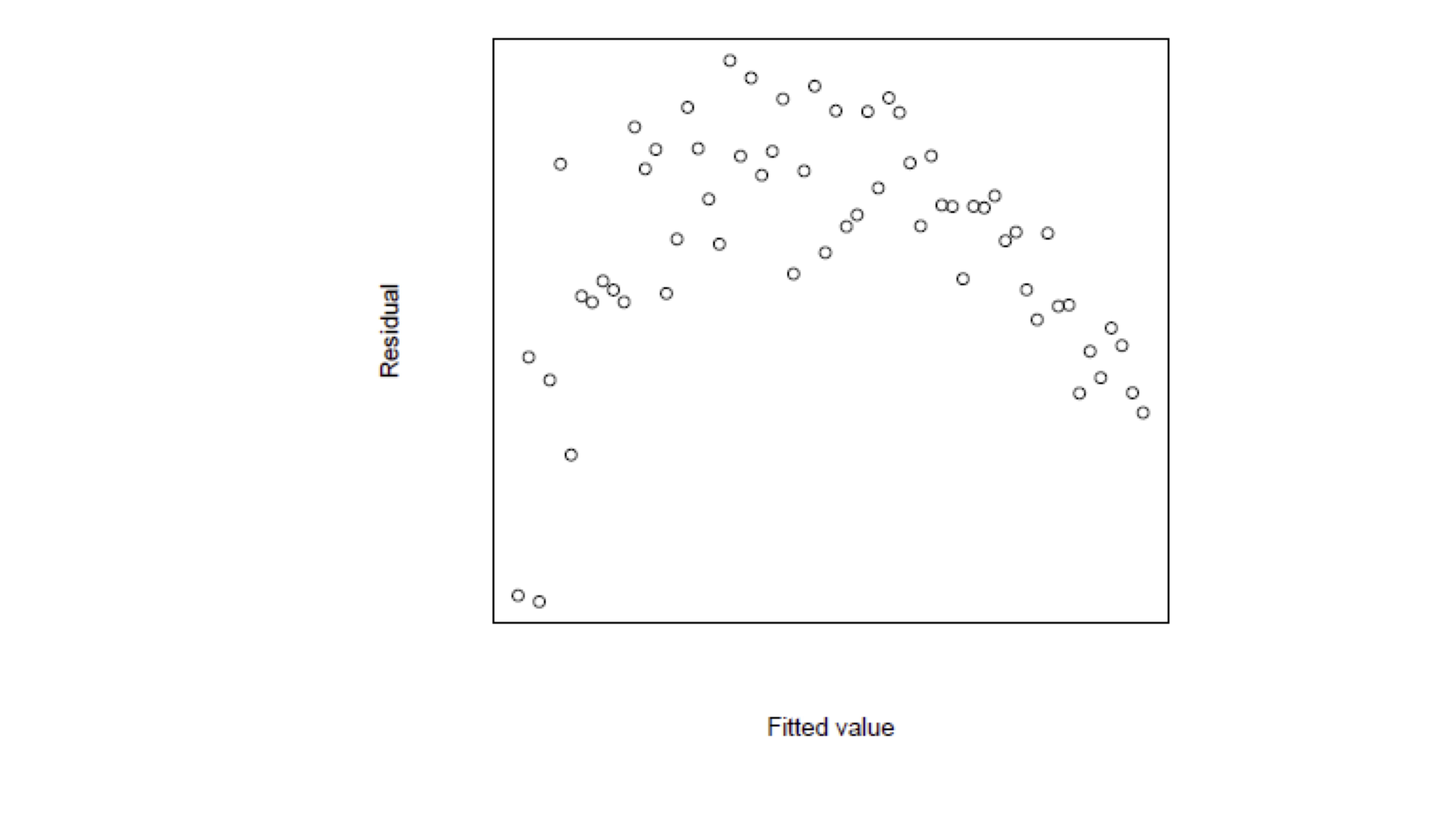
Funnelling in of residuals

Linear and Quadratic residuals

Remedial transformations

• To try and reduce heteroscedasticity we can
  • transform the data y
• A tranformation which often helps is
  • \, \log y
• For linear and quadratic patterns you can try
  • \, y^2
  • \, \sqrt{y}

Remedial transformations

• Heteroscedasticity can be associated with some of the X-variables

  • In this case plot the residuals or squared residuals against X

• The book [1] discusses two cases

  • The error variance is proportional to X^2_i {\rm Var}[\varepsilon_i] \, \approx \, \sigma^2 \, X^2_i
  • The error variance is proportional to X_i {\rm Var}[\varepsilon_i] \, \approx \, \sigma^2 \, X_i

• In each case divide through by the square root of the offending X-term

Error variance proportional to X_i^2

• Start with the model

Y_i = \beta_1 + \beta_2 X_{i} + \varepsilon_i

• Divide through by X_i

\begin{equation} \tag{1} \frac{Y_i}{X_i} = \frac{\beta_1}{X_i}+\beta_2+\frac{\varepsilon_i}{X_i} \end{equation}

• Estimate equation (1) with usual least squares regression approach

Error variance proportional to X_i

• Start with the model

Y_i = \beta_1 + \beta_2 X_{i} + \varepsilon_i

• Divide through by \sqrt{X_i}

\begin{equation} \tag{2} \frac{Y_i}{\sqrt{X_i}} = \frac{\beta_1}{\sqrt{X_i}}+\beta_2 \sqrt{X_i} + \frac{\varepsilon_i}{\sqrt{X_i}} \end{equation}

• Estimate equation (2) with usual least squares regression approach

Analysis of regression residuals in R

• We need R commands for residuals and fitted values

• Fit a linear model as usual

# Fit a linear model
model <- lm(formula)

• To obtain fitted values \hat y_i

# Compute fitted values
fitted.values <- model$fitted

• To obtain the residual values \varepsilon_i = y_i - \hat y_i

# Compute residual values
residuals <- model$resid

Example: Stock Vs Gold prices

• The full code for the example is available here residual_graphs.R

• Stock Vs Gold prices data is available here stock_gold.txt

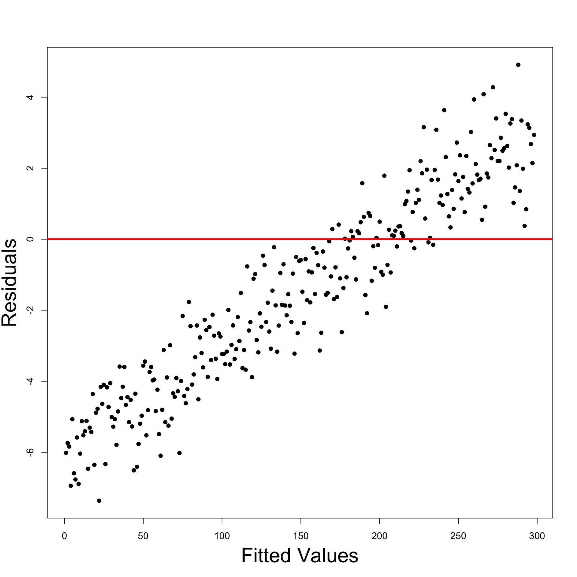
• Read data into R and fit simple regression

# Load dataset on Stock Vs Gold prices
prices <- read.table(file = "stock_gold.txt",
                    header = TRUE)

# Store data-frame into 2 vectors
stock.price <- prices[ , 1]
gold.price <- prices[ , 2]

# Fit regression model
model <- lm(gold.price ~ stock.price)

• Plot: Residuals look heteroscedastic
  • Most points are below the line
  • Points under the line appear more distant

# Scatter plot
plot(stock.price, 
     gold.price, 
     xlab = "Stock Price", 
     ylab = "Gold Price",
     pch = 16) 

# Plot regression line
abline(model, 
      col = "red", 
      lwd = 3)

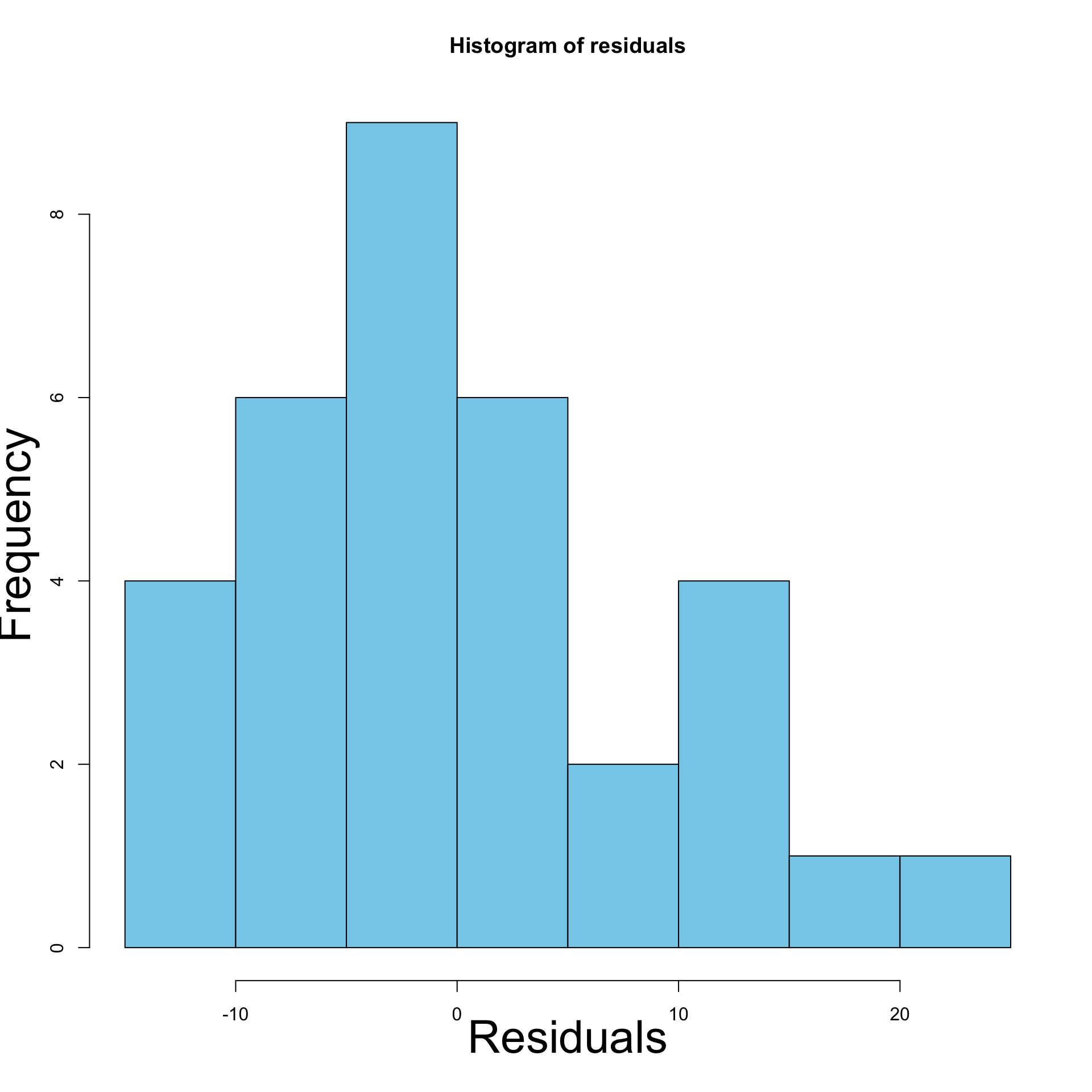
• Histogram: Confirms initial intuition of heteroscedasticity
  • Residuals are not normally distributed
  • Residuals have different variance (skewed histogram)

# Compute residuals
residuals <- model$resid

# Histogram of residuals
hist(residuals,
xlab = "Residuals",
ylab = "Frequency",
col = "skyblue")

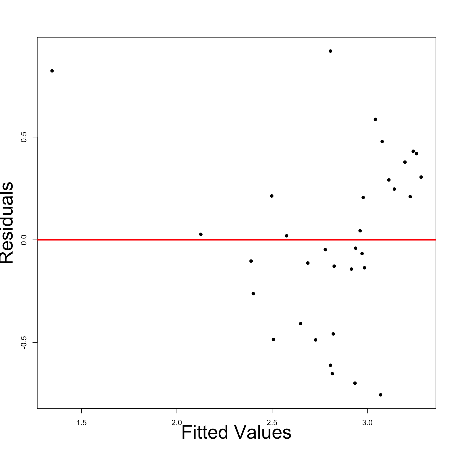
• Residual Graph: Displays funnelling out pattern
  • We definitely have heteroscedasticity

# Compute fitted values
fitted <- model$fitted

# Plot the residual graph
plot(fitted, residuals,
     xlab = "Fitted Values", 
     ylab = "Residuals",
     pch = 16)

# Add y = 0 line for reference
abline(0, 0, col = "red", lwd = 3)

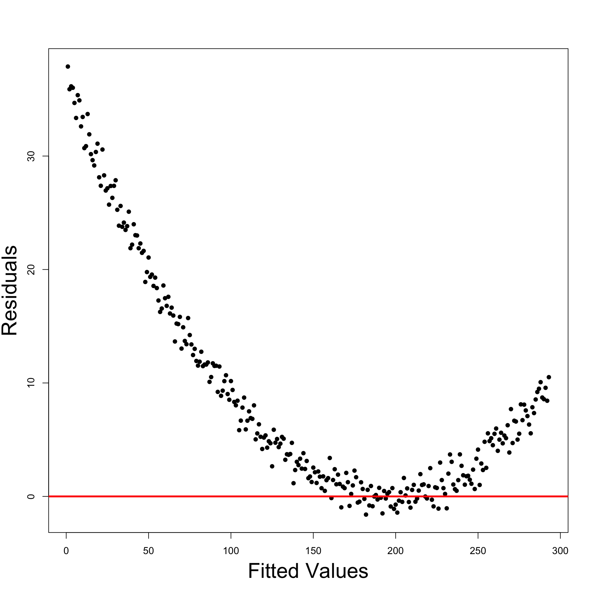
• Remedial transformation: To try and reduce heteroscedasticity take
  • \, \log y
• This means we need to fit the model

\log Y_i = \alpha + \beta X_i + \varepsilon_i

# Transform data via log(y)
log.gold.price <- log(gold.price)

# Fit linear model with log(y) data
log.model <- lm(log.gold.price ~ stock.price)

# Compute residuals for log model
log.residuals <- log.model$resid

# Compute fitted values for log model
log.fitted <- log.model$fitted

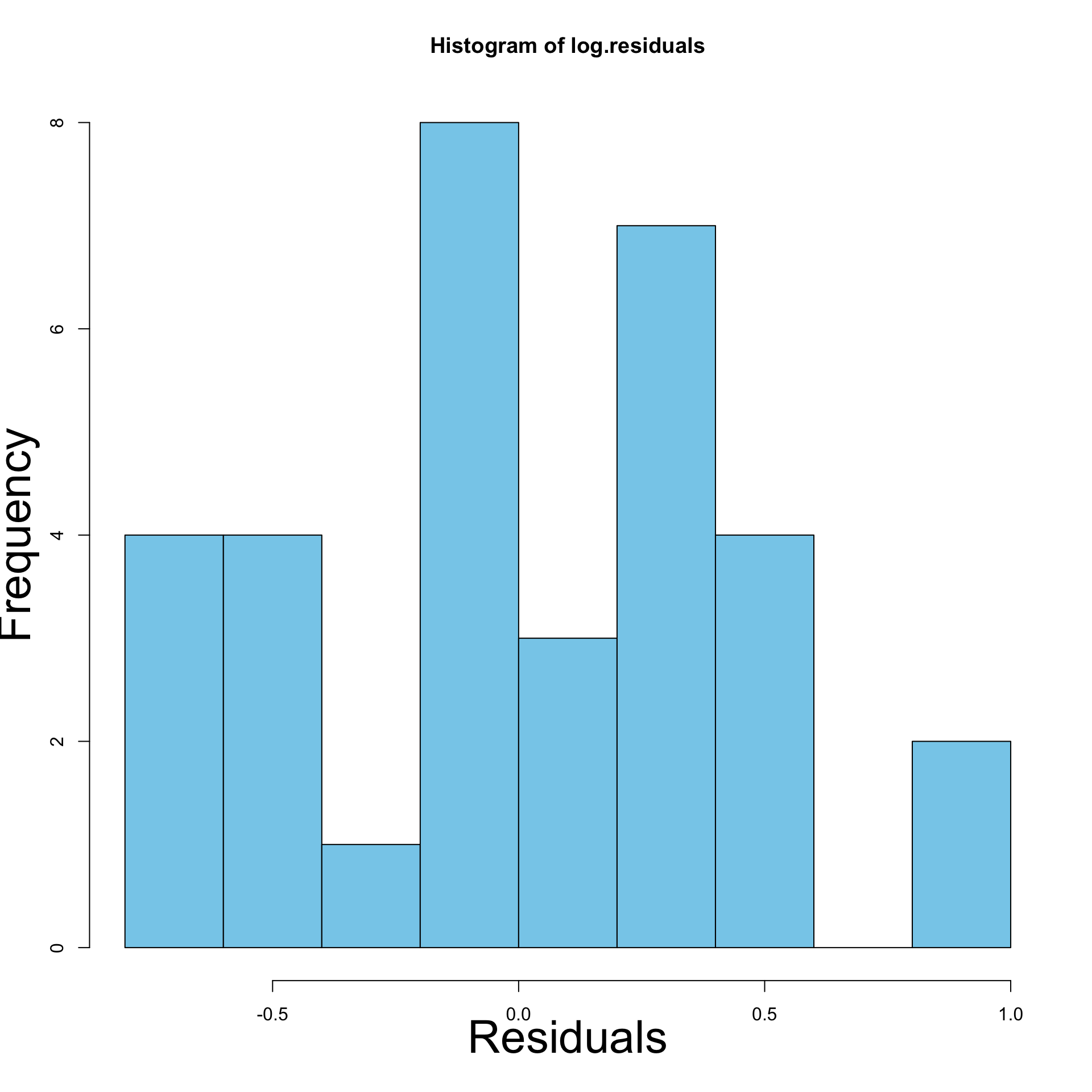
• Heteroscedasticity has definitely reduced
  • Left: Residual plot for original model
  • Right: Residual plot for \log y data model

• Heteroscedasticity has definitely reduced
  • Left: Histogram of residuals for original model
  • Right: Histogram of residuals for \log y data model

Part 2:
Autocorrelation

Autocorrelation

• The general linear regression model is

Y_i = \beta_1 z_{i1} + \beta_2 z_{i2} + \ldots + \beta_p z_{ip} + \varepsilon_i

• Consider Assumption 5
  • Independence: Errors \varepsilon_1, \ldots, \varepsilon_n are independent and thus uncorrelated {\rm Cor}(\varepsilon_i , \varepsilon_j) = 0 \qquad \forall \,\, i \neq j
• Autocorrelation: The violation of Assumption 5

{\rm Cor}(\varepsilon_i , \varepsilon_j) = 0 \qquad \text{ for some } \,\, i \neq j

Why is independence important?

• Recall the methods to assess linear models

  • Coefficient R^2
  • t-tests for parameters significance
  • F-test for model selection

• The above methods rely heavily on independence

Why is independence important?

• Once again let us consider the likelihood calculation \begin{align*} L & = f(y_1, \ldots, y_n) = \prod_{i=1}^n f_{Y_i} (y_i) \\[15pts] & = \frac{1}{(2\pi \sigma^2)^{n/2}} \, \exp \left( -\frac{\sum_{i=1}^n(y_i- \hat y_i)^2}{2\sigma^2} \right) \\[15pts] & = \frac{1}{(2\pi \sigma^2)^{n/2}} \, \exp \left( -\frac{ \mathop{\mathrm{RSS}}}{2\sigma^2} \right) \end{align*}

• The second equality is only possible thanks to independence of

Y_1 , \ldots, Y_n

Why is independence important?

• If we have autocorrelation then

{\rm Cor}(\varepsilon_i,\varepsilon_j) \neq 0 \quad \text{ for some } \, i \neq j

• In particualar we would have

\varepsilon_i \, \text{ and } \, \varepsilon_j \, \text{ dependent } \quad \implies \quad Y_i \, \text{ and } \, Y_j \, \text{ dependent }

• Therefore the calculation in previous slide breaks down

L \neq \frac{1}{(2\pi \sigma^2)^{n/2}} \, \exp \left( -\frac{ \mathop{\mathrm{RSS}}}{2\sigma^2} \right)

Why is independence important?

• In this case \hat \beta does no longer maximize the likelihood!

• As already seen, this implies that

\mathop{\mathrm{e.s.e.}}(\beta_j) \,\, \text{ is unreliable}

• Without independence the regression maths does not work!
  • t-tests for significance of \beta_j
  • confidence intervals for \beta_j
  • F-tests for model selection
  • They all break down and become unreliable!

Causes of Autocorrelation

Time-series data

• Autocorrelation means that

{\rm Cor}(\varepsilon_i,\varepsilon_j) \neq 0 \quad \text{ for some } \, i \neq j

• Autocorrelation if often unavoidable

• Typically associated with time series data

  • Observations ordered wrt time or space are usually correlated
  • This is because observations taken close together may take similar values

Causes of Autocorrelation

Financial data

• Autocorrelation is especially likely for datasets in
  • Accounting
  • Finance
  • Economics
• Autocorrelation is likely if the data have been recorded over time
  • E.g. daily, weekly, monthly, quarterly, yearly
• Example: Datasetet on Stock prices and Gold prices
  • General linear regression model assumes uncorrelated errors
  • Not realistic to assume that price observations for say 2020 and 2021 would be independent

Causes of Autocorrelation

Inertia

• Economic time series tend to exhibit cyclical behaviour

• Examples include GNP, price indices, production figures, employment statistics etc.

• Since these series tend to be quite slow moving

  • Effect of inertia is that successive observations are highly correlated

This is an extremely common phenomenon in financial and economic time series

Causes of Autocorrelation

Cobweb Phenomenon

• Characteristic of industries in which a large amount of time passes between

  • the decision to produce something
  • and its arrival on the market

• Cobweb phenomenon is common with agricultural commodities

• Economic agents (e.g. farmers) decide

  • how many goods to supply to the market
  • based on previous year price

Causes of Autocorrelation

Cobweb Phenomenon

• Example: the amount of crops farmers supply to the market at time t might be

\begin{equation} \tag{3} {\rm Supply}_t = \beta_1 + \beta_2 \, {\rm Price}_{t-1} + \varepsilon_t \end{equation}

• Errors \varepsilon_t in equation (3) are unlikely to be completely random and patternless

• This is because they represent actions of intelligent economic agents (e.g. farmers)

Error terms are likely to be autocorrelated

Causes of Autocorrelation

Data manipulation

Examples:

• Quarterly data may smooth out the wild fluctuations in monthly sales figures

• Low frequency economic survey data may be interpolated

However: Such data transformations may be inevitable

• In social sciences data quality may be variable

• This may induce systematic patterns and autocorrelation

No magic solution – Autocorrelation is unavoidable and must be considered

Detection of autocorrelation

• Statistical tests
  • Runs test
  • Durbin-Watson test
• Graphical methods
  • Simpler but can be more robust and more informative

Graphical and statistical methods can be useful cross-check of each other!

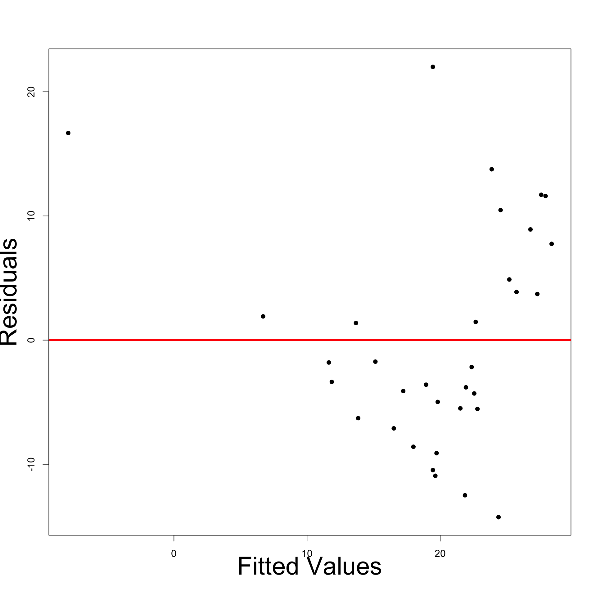
Graphical tests for autocorrelation

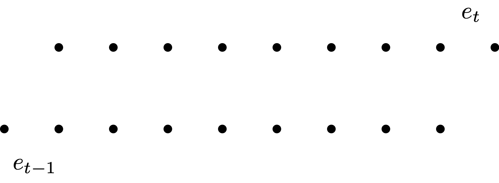
• Time-series plot of residuals
  • Plot residuals e_t over time
  • Check to see if any evidence of a systematic pattern exists
• Autocorrelation plot of residuals
  • Natural to think that \varepsilon_t and \varepsilon_{t-1} may be correlated
  • Plot residual e_t against e_{t-1}
• Important:
  • No Autocorrelation: Plots will look random
  • Yes Autocorrelation: Plots will show certain patterns

Graphical tests in R

• Code for this example is available here autocorrelation_graph_tests.R

• Stock Vs Gold prices data is available here stock_gold.txt

• Read data into R and fit simple regression

# Load dataset
prices <- read.table(file = "stock_gold.txt",
                    header = TRUE)

# Store data-frame into 2 vectors
stock.price <- prices[ , 1]
gold.price <- prices[ , 2]

# Fit regression model
model <- lm(gold.price ~ stock.price)

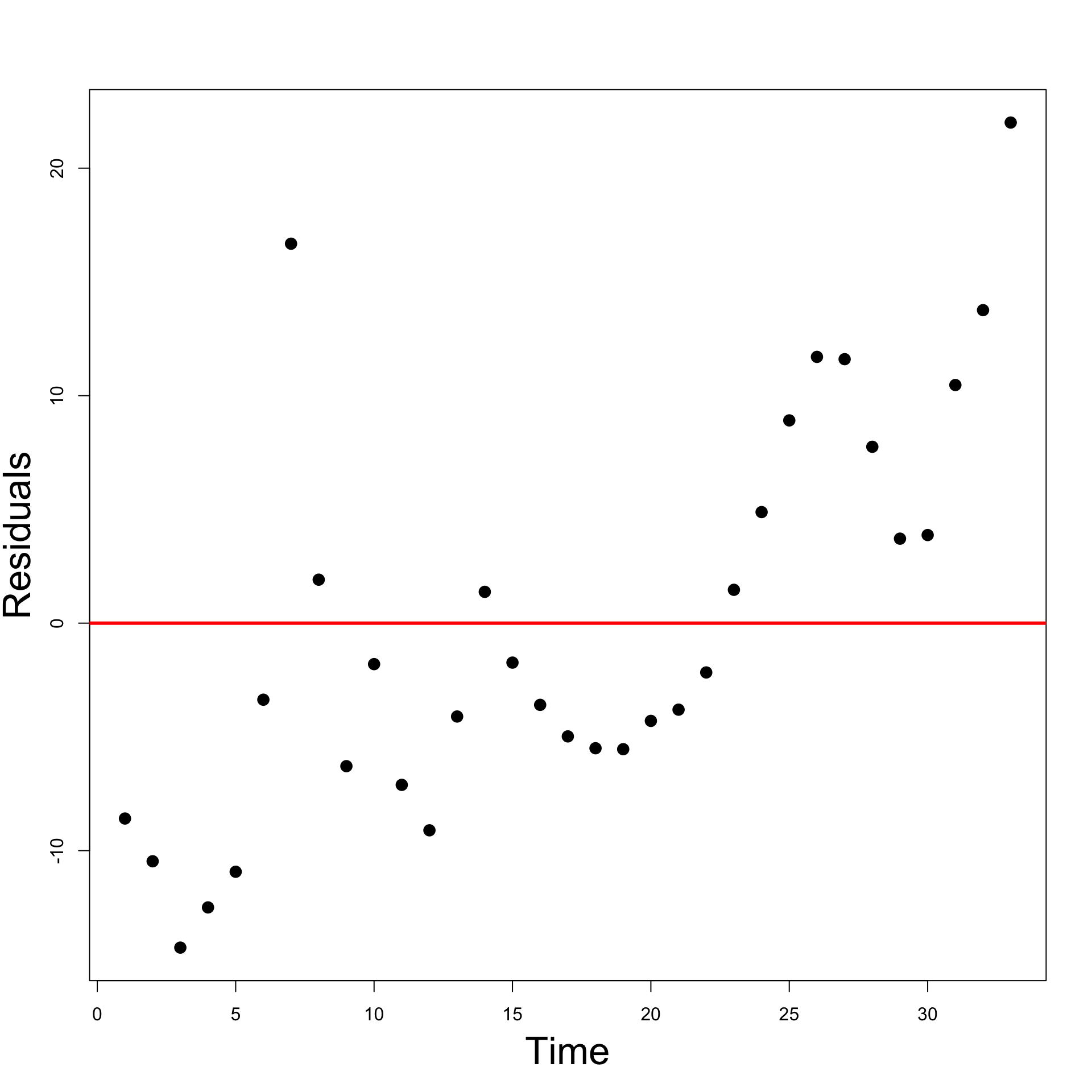
• Time-series plot of residuals
  • Time series plot suggests some evidence for autocorrelation
  • Look for successive runs of residuals either side of line y = 0 \, (see t = 15)

# Compute residuals
residuals <- model$resid

# Time-series plot of residuals
plot(residuals,
     xlab = "Time", 
     ylab = "Residuals",
     pch = 16,
     cex = 1.5)

# Add line y = 0 for reference
abline(0, 0, col = "red", lwd = 3)

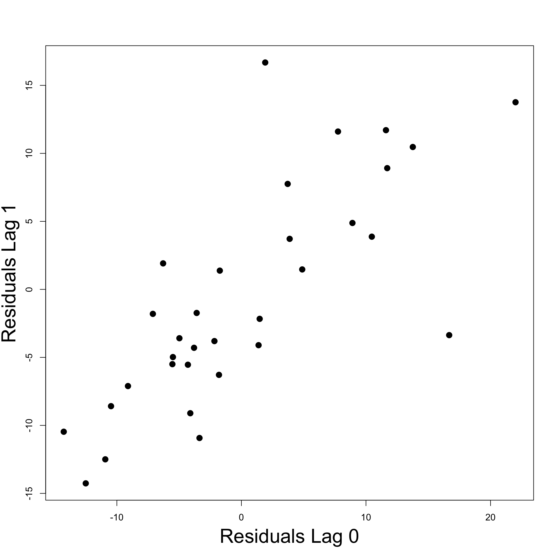
• Autocorrelation plot of residuals
  • Want to plot e_t against e_{t-1}
  • Shift e_t by 1 to get e_{t-1}
  • Can only plot magenta pairs
  • We have 1 pair less than number of residuals

• We want to plot e_t against e_{t-1}
  • Residuals are stored in vector \,\, \texttt{residuals}
  • We need to create a shifted version of \,\, \texttt{residuals}
  • First compute the length of \,\, \texttt{residuals}

# Compute length of residuals
length(residuals)

[1] 33

• Need to generate the 33-1 pairs for plotting

• Lag 0:
  • This is the original vector with no lag
  • Lose one observation from \,\, \texttt{residuals} – the first observation

residuals.lag.0 <- residuals[2:33]

• Lag 1:
  • This is the original vector shifted by 1
  • Lose one observation from \,\, \texttt{residuals} – the last observation

residuals.lag.1 <- residuals[1:32]

• Autocorrelation plot of residuals
  • Plot suggests positive autocorrelation of residuals
  • This means \, e_t \, \approx \, a + b \, e_{t-1} \, with b > 0

# Plot Lag0 Vs Lag1 residuals

plot(residuals.lag.0, 
     residuals.lag.1,
     xlab = "Residuals Lag 0", 
     ylab = "Residuals Lag 1",
     pch = 16,
     cex = 1.5)

Statistical tests for Autocorrelation

• Runs test
  • Under the classical multiple linear regression model residuals are equally likely to be positive or negative
• Durbin-Watson test
  • Test to see if residuals are AR(1)
• We do not cover these

What to do in case of Autocorrelation?

• Consider the simple regression model

Y_i = \alpha + \beta x_i + \varepsilon_i

• Suppose that autocorrelation occurs

{\rm Cor}(\varepsilon_i, \varepsilon_j ) \neq 0 \quad \text{ for some } \, i \neq j

• Also suppose that autocorrelation is linear in nature

e_t \, \approx \, a + b \, e_{t-1} \quad \text{ for some } \,\, a , \, b \in \mathbb{R}

• This was for example the case of Stock prices Vs Gold prices

What to do in case of Autocorrelation?

• In this case the simple linear model is not the right thing to consider

• The right thing to do is consider Autoregressive linear models

Y_t = \alpha + \beta x_{t} + \varepsilon_t

• These models couple regression with time-series analysis (ARIMA models)

• Good reference is book by Shumway and Stoffer [3]

Part 3:
Multicollinearity

Multicollinearity

• The general linear regression model is

Y_i = \beta_1 z_{i1} + \beta_2 z_{i2} + \ldots + \beta_p z_{ip} + \varepsilon_i

• Consider Assumption 6
  • The design matrix Z is such that Z^T Z \, \text{ is invertible}
• Multicollinearity: The violation of Assumption 6

\det(Z^T Z ) \, \approx \, 0 \, \quad \implies \quad Z^T Z \, \text{ is (almost) not invertible}

The nature of Multicollinearity

\text{Multicollinearity = multiple (linear) relationships between the Z-variables}

• Multicollinearity arises when there is either
  • exact linear relationship amongst the Z-variables
  • approximate linear relationship amongst the Z-variables

Z-variables inter-related \quad \implies \quad hard to isolate individual influence on Y

Example of Multicollinear data

• Perfect collinearity for Z_1 and Z_2

  • because of exact linear relation Z_2 = 5 Z_1

• No perfect collinearity for Z_1 and Z_3

• But Z_3 is small perturbation of Z_2

Z_1	Z_2	Z_3
10	50	52
15	75	75
18	90	97
24	120	129
30	150	152

Example of Multicollinear data

• Approximate collinearity for Z_1, Z_3
  • Correlation between Z_1 and Z_3 is almost 1
  • There is approximate linear relation between Z_1 and Z_3 Z_3 \, \approx \, 5 Z_1
• Both instances qualify as multicollinearity

Z_1	Z_2	Z_3
10	50	52
15	75	75
18	90	97
24	120	129
30	150	152

Example of Multicollinear data

# Enter the data
Z1 <- c(10, 15, 18, 24, 30)
Z3 <- c(52, 75, 97, 129, 152)

# Compute correlation
cor(Z1, Z3)

[1] 0.9958817

Z_1	Z_2	Z_3
10	50	52
15	75	75
18	90	97
24	120	129
30	150	152

Consequences of Multicollinearity

• Therefore multicollinearity means that
  • Predictors Z_j are (approximately) linearly dependent
  • E.g. one can be written as (approximate) linear combination of the others
• Recall that the design matrix is

Z = (Z_1 | Z_2 | \ldots | Z_p) = \left( \begin{array}{cccc} z_{11} & z_{12} & \ldots & z_{1p} \\ z_{21} & z_{22} & \ldots & z_{2p} \\ \ldots & \ldots & \ldots & \ldots \\ z_{n1} & z_{n2} & \ldots & z_{np} \\ \end{array} \right)

• Note that Z has p columns

Consequences of Multicollinearity

• If at least one pair Z_i and Z_j is collinear (linearly dependent) then

{\rm rank} (Z) < p

• Basic linear algebra tells us that

{\rm rank} \left( Z^T Z \right) = {\rm rank} \left( Z \right)

• Therefore if we have collinearity

{\rm rank} \left( Z^T Z \right) < p \qquad \implies \qquad Z^T Z \,\, \text{ is NOT invertible}

Consequences of Multicollinearity

• In this case the least-squares estimator is not well defined

\hat{\beta} = (Z^T Z)^{-1} Z^T y

Multicollinearity is a big problem!

Example of non-invertible Z^T Z

• Z_1, Z_2, Z_3 as before

• Exact Multicollinearity since Z_2 = 5 Z_1

• Thus Z^T Z is not invertible

• Let us check with R

Z_1	Z_2	Z_3
10	50	52
15	75	75
18	90	97
24	120	129
30	150	152

Example of non-invertible Z^T Z

# Enter the data
Z1 <- c(10, 15, 18, 24, 30)
Z2 <- c(50, 75, 90, 120, 150)
Z3 <- c(52, 75, 97, 129, 152)

# Assemble design matrix
Z <- matrix(c(Z1, Z2, Z3), ncol = 3)

# Compute determinant of Z^T Z
det ( t(Z) %*% Z )

[1] -3.531172e-07

Z_1	Z_2	Z_3
10	50	52
15	75	75
18	90	97
24	120	129
30	150	152

Example of non-invertible Z^T Z

• R computed that \,\, {\rm det} ( Z^T Z) = -3.531172 \times 10^{-7}

• Therefore the determinant of Z^T Z is almost 0

Z^T Z \text{ is not invertible!}

• If we try to invert Z^T Z in R we get an error

# Compute inverse of Z^T Z
solve ( t(Z) %*% Z )

Error in solve.default(t(Z) %*% Z) : 
  system is computationally singular: reciprocal condition number = 8.25801e-19

Approximate Multicollinearity

• In practice one almost never has exact Multicollinearity

• If Multicollinearity is present, it is likely to be Approximate Multicollinearity

• In case of approximate Multicollinearity it holds that

  • The matrix Z^T Z can be inverted
  • The estimator \hat \beta can be computed \hat \beta = (Z^T Z)^{-1} Z^T y
  • However the inversion is numerically instable

Approximate Multicollinearity is still a big problem!

Numerical instability

• Numerical instability means that:
  • We may not be able to trust the estimator \hat \beta

This is because of:

1. Larger estimated standard errors
   • Lack of precision associated with parameter estimates
   • Wider confidence intervals
   • May affect hypothesis tests
2. Correlated parameter estimates
   • Another potential source of errors
   • Potential numerical problems with computational routines

The effects of numerical instability

• Approximate Multicollinearity implies that
  • Z^T Z is invertible
  • The inversion is numerically instable
• Numerically instable inversion means that

\text{Small perturbations in } Z \quad \implies \quad \text{large variations in } (Z^T Z)^{-1}

• Denote by \xi_{ij} the entries of (Z^T Z)^{-1}

\text{Small perturbations in } Z \quad \implies \quad \text{large variations in } \xi_{ij}

• This in particular might lead to larger than usual values \xi_{ij}

Why are estimated standard errors larger?

• Recall formula of estimated standard error for \beta_j

\mathop{\mathrm{e.s.e.}}(\beta_j) = \xi_{jj}^{1/2} \, S \,, \qquad \quad S^2 = \frac{\mathop{\mathrm{RSS}}}{n-p}

• The numbers \xi_{jj} are the diagonal entries of (Z^T Z)^{-1}

\begin{align*} \text{Multicollinearity} & \quad \implies \quad \text{Numerical instability} \\[5pts] & \quad \implies \quad \text{potentially larger } \xi_{jj} \\[5pts] & \quad \implies \quad \text{potentially larger } \mathop{\mathrm{e.s.e.}}(\beta_j) \end{align*}

• It becomes harder to reject incorrect hypotheses

Effect of Multicollinearity on t-tests

• To test the null hypothesis that \beta_j = 0 we use t-statistic

t = \frac{\beta_j}{ \mathop{\mathrm{e.s.e.}}(\beta_j) }

• But Multicollinearity increases the \mathop{\mathrm{e.s.e.}}(\beta_j)

• Therefore the t-statistic reduces in size:

  • t-statistic will be smaller than it should
  • The p-values will be large p > 0.05

It becomes harder to reject incorrect hypotheses!

Example of numerical instability

• Z_1, Z_2, Z_3 as before

• We know we have exact Multicollinearity, since Z_2 = 5 Z_1

• Therefore Z^T Z is not invertible

Z_1	Z_2	Z_3
10	50	52
15	75	75
18	90	97
24	120	129
30	150	152

Example of numerical instability

• To get rid of Multicollinearity we can add a small perturbation to Z_1 Z_1 \,\, \leadsto \,\, Z_1 + 0.01

• The new dataset Z_1 + 0.01, Z_2, Z_3 is

  • Not anymore exactly Multicollinear
  • Still approximately Multicollinear

Z_1	Z_2	Z_3
10	50	52
15	75	75
18	90	97
24	120	129
30	150	152

Example of numerical instability

• Define the new design matrix Z = (Z_1 + 0.01 | Z_2 | Z_3)

• Data is approximately Multicollinear

• Therefore the inverse of Z^T Z exists

• Let us compute this inverse in R

Z_1 + 0.01	Z_2	Z_3
10.01	50	52
15.01	75	75
18.01	90	97
24.01	120	129
30.01	150	152

• Let us compute the inverse of

Z = (Z_1 + 0.01 | Z_2 | Z_3)

# Consider perturbation Z1 + 0.01
PZ1 <- Z1 + 0.01

# Assemble perturbed design matrix
Z <- matrix(c(PZ1, Z2, Z3), ncol = 3)

# Compute the inverse of Z^T Z
solve ( t(Z) %*% Z )

             [,1]          [,2]       [,3]
[1,] 17786.804216 -3556.4700048 -2.4186075
[2,] -3556.470005   711.1358432  0.4644159
[3,]    -2.418608     0.4644159  0.0187805

• In particular note that the first coefficient is \,\, \xi_{11} \, \approx \, 17786

• Let us change the perturbation slightly:

\text{ consider } \, Z_1 + 0.02 \, \text{ instead of } \, Z_1 + 0.01

• Invert the new design matrix \,\, Z = (Z_1 + 0.02 | Z_2 | Z_3)

# Consider perturbation Z1 + 0.02
PZ1 <- Z1 + 0.02

# Assemble perturbed design matrix
Z <- matrix(c(PZ1, Z2, Z3), ncol = 3)

# Compute the inverse of Z^T Z
solve ( t(Z) %*% Z )

            [,1]         [,2]       [,3]
[1,] 4446.701047 -888.8947902 -1.2093038
[2,] -888.894790  177.7098841  0.2225551
[3,]   -1.209304    0.2225551  0.0187805

• In particular note that the first coefficient is \,\, \xi_{11} \, \approx \, 4446

• Summary:
  • If we perturb the vector Z_1 by 0.01 the first coefficient of Z^T Z is \xi_{11} \, \approx \, 17786
  • If we perturb the vector Z_1 by 0.02 the first coefficient of Z^T Z is \xi_{11} \, \approx \, 4446

• Note that the average entry in Z_1 is

mean(Z1)

[1] 19.4

• Therefore the average percentage change in the data is

\begin{align*} \text{Percentage Change} & = \left( \frac{\text{New Value} - \text{Old Value}}{\text{Old Value}} \right) \times 100\% \\[15pts] & = \left( \frac{(19.4 + 0.02) - (19.4 + 0.01)}{19.4 + 0.01} \right) \times 100 \% \ \approx \ 0.05 \% \end{align*}

• The percentage change in the coefficients \xi_{11} is

\text{Percentage Change in } \, \xi_{11} = \frac{4446 - 17786}{17786} \times 100 \% \ \approx \ −75 \%

• Conclusion: We have shown that

\text{perturbation of } \, 0.05 \% \, \text{ in the data } \quad \implies \quad \text{change of } \, - 75 \% \, \text{ in } \, \xi_{11}

• This is precisely numerical instability

\text{Small perturbations in } Z \quad \implies \quad \text{large variations in } (Z^T Z)^{-1}

Sources of Multicollinearity

• Multicollinearity is a problem
  • When are we likely to encounter it?
• Possible sources of Multicollinearity are

1. The data collection method employed
   • Sampling over a limited range of values taken by the regressors in the population
2. Constraints on the model or population
   • E.g. variables such as income and house size may be interrelated
3. Model Specification
   • E.g. adding polynomial terms to a model when range of X-variables is small

Sources of Multicollinearity

4. An over-determined model
   • Having too many X variables compared to the number of observations
5. Common trends
   • E.g. variables such as consumption, income, wealth, etc may be correlated due to a dependence upon general economic trends and cycles

Often can know in advance when you might experience Multicollinearity

How to detect Multicollinearity in practice?

Most important sign

• In practical problems look for something that does not look quite right

Important

High R^2 values coupled with small t-values

• This is a big sign of potential Multicollinearity

• Why is this contradictory?

  • High R^2 suggests model is good and explains a lot of the variation in Y
  • But if individual t-statistics are small, this suggests \beta_j = 0
  • Hence individual X-variables do not affect Y

How to detect Multicollinearity in practice?

Other signs of Multicollinearity

Numerical instabilities:

• Parameter estimates \hat \beta_j become very sensitive to small changes in the data

• The \mathop{\mathrm{e.s.e.}} become very sensitive to small changes in the data

• Parameter estimates \hat \beta_j take the wrong sign or otherwise look strange

• Parameter estimates may be highly correlated

Example of Multicollinearity

• Consider the following illustrative example

• Want to explain expenditure Y in terms of

  • income X_2
  • wealth X_3

• It is intuitively clear that income and wealth are highly correlated

Important

To detect Multicollinearity look out for

• High R^2 value
• coupled with low t-values

Example dataset

Expenditure Y	Income X_2	Wealth X_3
70	80	810
65	100	1009
90	120	1273
95	140	1425
110	160	1633
115	180	1876
120	200	2052
140	220	2201
155	240	2435
150	260	2686

Fit the regression model in R

• Code for this example is available here multicollinearity.R

# Enter data
y <- c(70, 65, 90, 95, 110, 115, 120, 140, 155, 150)
x2 <- c(80, 100, 120, 140, 160, 180, 200, 220, 240, 260)
x3 <- c(810, 1009, 1273, 1425, 1633, 1876, 2052, 2201, 2435, 2686)

# Fit model
model <- lm(y ~ x2 + x3)

# We want to display only part of summary
# First capture the output into a vector
temp <- capture.output(summary(model))

# Then print only the lines of interest
cat(paste(temp[9:20], collapse = "\n"))

Coefficients:
            Estimate Std. Error t value Pr(>|t|)   
(Intercept) 24.77473    6.75250   3.669  0.00798 **
x2           0.94154    0.82290   1.144  0.29016   
x3          -0.04243    0.08066  -0.526  0.61509   
---
Signif. codes:  0 '***' 0.001 '**' 0.01 '*' 0.05 '.' 0.1 ' ' 1

Residual standard error: 6.808 on 7 degrees of freedom
Multiple R-squared:  0.9635,    Adjusted R-squared:  0.9531 
F-statistic:  92.4 on 2 and 7 DF,  p-value: 9.286e-06

Three basic statistics

• R^2 coefficient
• t-statistics and related p-values
• F-statistic and related p-value

Interpreting the R output

1. R^2 = 0.9635
   • Model explains a substantial amount of the variation (96.35%) in the data

2. F-statistic is
   • F = 92.40196
   • Corresponding p-value is p = 9.286 \times 10^{-6}
   • There is evidence p<0.05 that at least one between income and wealth affect expenditure

Interpreting the R output

3. t-statistics
   • t-statistics for income is t = 1.144
   • Corresponding p-value is p = 0.29016
   • t-statistic for wealth is t = -0.526
   • Corresponding p-value is p = 0.61509
   • Both p-values are p > 0.05
   • Therefore neither income nor wealth are individually statistically significant
   • This means regression parameters are \beta_2 = \beta_3 = 0

Main red flag for Multicollinearity:

• High R^2 value coupled with low t-values (corresponding to high p-values)

The output looks strange

There are many contradictions

1. High R^2 value suggests model is really good

2. However low t-values imply neither income nor wealth affect expenditure

3. F-statistic is high, meaning that at least one between income nor wealth affect expenditure

4. The wealth variable has the wrong sign (\hat \beta_3 < 0)

   • This makes no sense: it is likely that expenditure will increase as wealth increases
   • Therefore we would expect \, \hat \beta_3 > 0

Multicollinearity is definitely present!

Detection of Multicollinearity

Computing the correlation

• For further confirmation of Multicollinearity compute correlation of X_2 and X_3

cor(x2, x3)

[1] 0.9989624

• Correlation is almost 1: Variables X_2 and X_3 are very highly correlated

This once again confirms Multicollinearity is present

Conclusion: The variables Income and Wealth are highly correlated

• Impossible to isolate individual impact of either Income or Wealth upon Expenditure

Detection of Multicollinearity

Klein’s rule of thumb

Klein’s rule of thumb: Multicollinearity will be a serious problem if:

• The R^2 obtained from regressing predictor variables X is greater than the overall R^2 obtained by regressing Y against all the X variables

Example: In the Expenditure vs Income and Wealth dataset we have

• Regressing Y against X_2 and X_3 gives R^2=0.9635

• Regressing X_2 against X_3 gives R^2 = 0.9979

Klein’s rule of thumb suggests that Multicollinearity will be a serious problem

Remedial measures

Do nothing

• Multicollinearity is essentially a data-deficiency problem

• Sometimes we have no control over the dataset available

• Important point:

  • Doing nothing should only be an option in quantitative social sciences (e.g. finance, economics) where data is often difficult to collect
  • For scientific experiments (e.g. physics, chemistry) one should strive to collect good data

Remedial measures

Acquire new/more data

• Multicollinearity is a sample feature

• Possible that another sample involving the same variables will have less Multicollinearity

• Acquiring more data might reduce severity of Multicollinearity

• More data can be collected by either

  • increasing the sample size or
  • including additional variables

Remedial measures

Use prior information about some parameters

• To do this properly would require advanced Bayesian statistical methods

• This is beyond the scope of this module

Remedial measures

Rethinking the model

• Sometimes a model chosen for empirical analysis is not carefully thought out
  • Some important variables may be omitted
  • The functional form of the model may have been incorrectly chosen
• Sometimes using more advanced statistical techniques may be required
  • Factor Analysis
  • Principal Components Analysis
  • Ridge Regression
• Above techniques are outside the scope of this module

Remedial measures

Transformation of variables

• Multicollinearity may be reduced by transforming variables

• This may be possible in various different ways

  • E.g. for time-series data one might consider forming a new model by taking first differences

• Further reading in Chapter 10 of [1]

Remedial measures

Dropping variables

• Simplest approach to tackle Multicollinearity is to drop one or more of the collinear variables

• Goal: Find the best combination of X variables which reduces Multicollinearity

• We present 2 alternatives

  1. Dropping variables by hand
  2. Dropping variables using Stepwise regression

Example: Dropping variables by hand

• Consider again the Expenditure vs Income and Wealth dataset

• The variables Income and Wealth are highly correlated

• Intuitively we expect both Income and Wealth to affect Expenditure

• Solution can be to drop either Income or Wealth variables

  • We can then fit 2 separate models

# Fit expenditure as function of income
model.1 <- lm(y ~ x2)

# Fit expenditure as function of wealth
model.2 <- lm(y ~ x3)

summary(model.1)
summary(model.2)

Expenditure Vs Income

Coefficients:
            Estimate Std. Error t value Pr(>|t|)    
(Intercept) 24.45455    6.41382   3.813  0.00514 ** 
x2           0.50909    0.03574  14.243 5.75e-07 ***
---
Signif. codes:  0 '***' 0.001 '**' 0.01 '*' 0.05 '.' 0.1 ' ' 1

Residual standard error: 6.493 on 8 degrees of freedom
Multiple R-squared:  0.9621,    Adjusted R-squared:  0.9573 
F-statistic: 202.9 on 1 and 8 DF,  p-value: 5.753e-07

• R^ 2 = 0.9621 which is quite high
• p-value for \beta_2 is p = 9.8 \times 10^{-7} < 0.5 \quad \implies \quad Income variable is significant
• Estimate is \hat \beta_2 = 0.50909 > 0

Strong evidence that Expenditure increases as Income increases

Expenditure Vs Wealth

Coefficients:
             Estimate Std. Error t value Pr(>|t|)    
(Intercept) 24.411045   6.874097   3.551   0.0075 ** 
x3           0.049764   0.003744  13.292  9.8e-07 ***
---
Signif. codes:  0 '***' 0.001 '**' 0.01 '*' 0.05 '.' 0.1 ' ' 1

Residual standard error: 6.938 on 8 degrees of freedom
Multiple R-squared:  0.9567,    Adjusted R-squared:  0.9513 
F-statistic: 176.7 on 1 and 8 DF,  p-value: 9.802e-07

• R^ 2 = 0.9567 which is quite high
• p-value for \beta_2 is p = 9.8 \times 10^{-7} < 0.5 \quad \implies \quad Wealth variable is significant
• Estimate is \hat \beta_2 = 0.049764 > 0

Strong evidence that Expenditure increases as Wealth increases

Example: Conclusion

• We considered the simpler models
  • Expenditure vs Income
  • Expenditure vs Wealth
• Both models perform really well
  • Expenditure increases as either Income or Wealth increase
• Multicollinearity effects disappeared after dropping either variable!

Stepwise regression

• Stepwise regression: Method of comparing regression models

• Involves iterative selection of predictor variables X to use in the model

• It can be achieved through

  • Forward selection
  • Backward selection
  • Stepwise selection: Combination of Forward and Backward selection

Stepwise regression methods

1. Forward Selection
   • Start with the null model with only intercept Y = \beta_1 + \varepsilon
   • Add each variable X_j incrementally, testing for significance
   • Stop when no more variables are statistically significant

Note: Significance criterion for X_j is in terms of AIC

• AIC is a measure of how well a model fits the data
• AIC is an alternative to the coefficient of determination R^2
• We will give details about AIC later

Stepwise regression methods

2. Backward Selection
   • Start with the full model Y = \beta_1 + \beta_2 X_{2}+ \ldots+\beta_p X_{p}+ \varepsilon
   • Delete X_j variables which are not significant
   • Stop when all the remaining variables are significant

Stepwise regression methods

3. Stepwise Selection
   • Start with the null model Y = \beta_1 + \varepsilon
   • Add each variable X_j incrementally, testing for significance
   • Each time a new variable X_j is added, perform a Backward Selection step
   • Stop when all the remaining variables are significant

Note: Stepwise Selection ensures that at each step all the variables are significant

Stepwise regression in R

• Suppose given
  • a data vector \, \texttt{y}
  • predictors data \, \texttt{x2}, \texttt{x3}, \ldots, \texttt{xp}

• Begin by fitting the null and full regression models

# Fit the null model
null.model <- lm(y ~ 1)

# Fit the full model
full.model <- lm(y ~ x2 + x3 + ... + xp)

Stepwise regression in R

• There are 2 basic differences depending on whether you are doing
  • Forward selection or Stepwise selection: Start with null model
  • Backward selection: Start with full model

• The command for Stepwise selection is

# Stepwise selection
best.model <- step(null.model, 
                   direction = "both", 
                   scope = formula(full.model))

Stepwise regression in R

• The command for Forward selection is

# Forward selection
best.model <- step(null.model, 
                   direction = "forward", 
                   scope = formula(full.model))

• The command for Backward selection is

# Backward selection
best.model <- step(full.model, 
                   direction = "backward")

Stepwise regression in R

• The model selected by Stepwise regression is saved in
  • \texttt{best.model}

• To check which model is best, just print the summary and read first 2 lines

summary(best.model)

Example: Longley dataset

      GNP Unemployed Armed.Forces Population Year Employed
1 234.289      235.6        159.0    107.608 1947   60.323
2 259.426      232.5        145.6    108.632 1948   61.122
3 258.054      368.2        161.6    109.773 1949   60.171

Goal: Explain the number of Employed people Y in the US in terms of

• X_2 GNP Gross National Product
• X_3 number of Unemployed
• X_4 number of people in the Armed Forces
• X_5 non-institutionalised Population \geq age 14 (not in care of insitutions)
• X_6 Years from 1947 to 1962

Reading in the data

• Code for this example is available here longley_stepwise.R

• Longley dataset available here longley.txt

• Download the data file and place it in current working directory

# Read data file
longley <- read.table(file = "longley.txt",
                      header = TRUE)

# Store columns in vectors
x2 <- longley[ , 1]
x3 <- longley[ , 2]
x4 <- longley[ , 3]
x5 <- longley[ , 4]
x6 <- longley[ , 5]
y <- longley[ , 6]

Detecting Multicollinearity

• Fit the multiple regression model including all predictors

Y = \beta_1 + \beta_2 \, X_2 + \beta_3 \, X_3 + \beta_4 \, X_4 + \beta_5 \, X_5 + \beta_6 \, X_6 + \varepsilon

# Fit multiple regression model
model <- lm(y ~ x2 + x3 + x4 + x5 + x6)

# Print summary
summary(model)

• Fitting the full model gives
  • High R^2 value
  • Low t-values (and high p-values) for X_2 and X_5
• These are signs that we might have a problem with Multicollinearity

• To further confirm Multicollinearity we can look at the correlation matrix
  • We can use function \, \texttt{cor} directly on first 5 columns of data-frame \,\texttt{longley}
  • We look only at correlations larger than 0.9

# Return correlations larger than 0.9
cor(longley[ , 1:5]) > 0.9

               GNP Unemployed Armed.Forces Population  Year
GNP           TRUE      FALSE        FALSE       TRUE  TRUE
Unemployed   FALSE       TRUE        FALSE      FALSE FALSE
Armed.Forces FALSE      FALSE         TRUE      FALSE FALSE
Population    TRUE      FALSE        FALSE       TRUE  TRUE
Year          TRUE      FALSE        FALSE       TRUE  TRUE

• Hence the following pairs are highly correlated (correlation \, > 0.9) X_2 \,\, \text{and} \,\, X_5 \qquad \quad X_2 \,\, \text{and} \,\, X_6 \qquad \quad X_4 \,\, \text{and} \,\, X_6

Applying Stepwise regression

• Goal: Want to find best variables which, at the same time
  • Explain Employment variable Y
  • Reduce Multicollinearity
• Method: We use Stepwise regression

• Start by by fitting the null and full regression models

# Fit the null model
null.model <- lm(y ~ 1)

# Fit the full model
full.model <- lm(y ~ x2 + x3 + x4 + x5 + x6)

Applying Stepwise regression

• Perform Stepwise regression by
  • Forward selection, Backward selection, Stepwise selection

# Forward selection
best.model.1 <- step(null.model, 
                    direction = "forward", 
                    scope = formula(full.model))

# Backward selection
best.model.2 <- step(full.model, 
                    direction = "backward")

# Stepwise selection
best.model.3 <- step(null.model, 
                    direction = "both",
                    scope = formula(full.model))

Applying Stepwise regression

• Models obtained by Stepwise regression are stored in
  • \texttt{best.model.1}, \,\, \texttt{best.model.3}, \,\,\texttt{best.model.3}

• Print the summary for each model obtained

# Print summary of each model
summary(best.model.x)

• Output: The 3 methods all yield the same model

Call:
lm(formula = y ~ x2 + x3 + x4 + x6)

Interpretation

• All three Stepwise regression methods agree and select a model with the variables
  • X_2, X_3, X_4 and X_6
  • X_5 is excluded
• Explanation: Multicollinearity and inter-relationships between the X-variables mean that there is some redundancy
  • the X_5 variable is not needed in the model
• This means that the number Employed just depends on
  • X_2 GNP
  • X_3 Number of Unemployed people
  • X_4 Number of people in the Armed Forces
  • X_6 Time in Years

Re-fitting the model without X_5

Call:
lm(formula = y ~ x2 + x3 + x4 + x6)

Coefficients:
              Estimate Std. Error t value Pr(>|t|)    
(Intercept) -3.599e+03  7.406e+02  -4.859 0.000503 ***
x2          -4.019e-02  1.647e-02  -2.440 0.032833 *  
x3          -2.088e-02  2.900e-03  -7.202 1.75e-05 ***
x4          -1.015e-02  1.837e-03  -5.522 0.000180 ***
x6           1.887e+00  3.828e-01   4.931 0.000449 ***
---
Signif. codes:  0 ‘***’ 0.001 ‘**’ 0.01 ‘*’ 0.05 ‘.’ 0.1 ‘ ’ 1

Residual standard error: 0.2794 on 11 degrees of freedom
Multiple R-squared:  0.9954,    Adjusted R-squared:  0.9937 
F-statistic: 589.8 on 4 and 11 DF,  p-value: 9.5e-13

• Coefficient of determination is still very high: R^2 = 0.9954
• All the variables X_2, X_3,X_4,X_6 are significant (high t-values)
• This means Multicollinearity effects have disappeared

Re-fitting the model without X_5

Call:
lm(formula = y ~ x2 + x3 + x4 + x6)

Coefficients:
              Estimate Std. Error t value Pr(>|t|)    
(Intercept) -3.599e+03  7.406e+02  -4.859 0.000503 ***
x2          -4.019e-02  1.647e-02  -2.440 0.032833 *  
x3          -2.088e-02  2.900e-03  -7.202 1.75e-05 ***
x4          -1.015e-02  1.837e-03  -5.522 0.000180 ***
x6           1.887e+00  3.828e-01   4.931 0.000449 ***
---
Signif. codes:  0 ‘***’ 0.001 ‘**’ 0.01 ‘*’ 0.05 ‘.’ 0.1 ‘ ’ 1

Residual standard error: 0.2794 on 11 degrees of freedom
Multiple R-squared:  0.9954,    Adjusted R-squared:  0.9937 
F-statistic: 589.8 on 4 and 11 DF,  p-value: 9.5e-13

• The coefficient of X_2 is negative and statistically significant
  • As GNP increases the number Employed decreases

Re-fitting the model without X_5

Call:
lm(formula = y ~ x2 + x3 + x4 + x6)

Coefficients:
              Estimate Std. Error t value Pr(>|t|)    
(Intercept) -3.599e+03  7.406e+02  -4.859 0.000503 ***
x2          -4.019e-02  1.647e-02  -2.440 0.032833 *  
x3          -2.088e-02  2.900e-03  -7.202 1.75e-05 ***
x4          -1.015e-02  1.837e-03  -5.522 0.000180 ***
x6           1.887e+00  3.828e-01   4.931 0.000449 ***
---
Signif. codes:  0 ‘***’ 0.001 ‘**’ 0.01 ‘*’ 0.05 ‘.’ 0.1 ‘ ’ 1

Residual standard error: 0.2794 on 11 degrees of freedom
Multiple R-squared:  0.9954,    Adjusted R-squared:  0.9937 
F-statistic: 589.8 on 4 and 11 DF,  p-value: 9.5e-13

• The coefficient of X_3 is negative and statistically significant
  • As the number of Unemployed increases the number Employed decreases

Re-fitting the model without X_5

Call:
lm(formula = y ~ x2 + x3 + x4 + x6)

Coefficients:
              Estimate Std. Error t value Pr(>|t|)    
(Intercept) -3.599e+03  7.406e+02  -4.859 0.000503 ***
x2          -4.019e-02  1.647e-02  -2.440 0.032833 *  
x3          -2.088e-02  2.900e-03  -7.202 1.75e-05 ***
x4          -1.015e-02  1.837e-03  -5.522 0.000180 ***
x6           1.887e+00  3.828e-01   4.931 0.000449 ***
---
Signif. codes:  0 ‘***’ 0.001 ‘**’ 0.01 ‘*’ 0.05 ‘.’ 0.1 ‘ ’ 1

Residual standard error: 0.2794 on 11 degrees of freedom
Multiple R-squared:  0.9954,    Adjusted R-squared:  0.9937 
F-statistic: 589.8 on 4 and 11 DF,  p-value: 9.5e-13

• The coefficient of X_4 is negative and statistically significant
  • As the number of Armed Forces increases the number Employed decreases

Re-fitting the model without X_5

Call:
lm(formula = y ~ x2 + x3 + x4 + x6)

Coefficients:
              Estimate Std. Error t value Pr(>|t|)    
(Intercept) -3.599e+03  7.406e+02  -4.859 0.000503 ***
x2          -4.019e-02  1.647e-02  -2.440 0.032833 *  
x3          -2.088e-02  2.900e-03  -7.202 1.75e-05 ***
x4          -1.015e-02  1.837e-03  -5.522 0.000180 ***
x6           1.887e+00  3.828e-01   4.931 0.000449 ***
---
Signif. codes:  0 ‘***’ 0.001 ‘**’ 0.01 ‘*’ 0.05 ‘.’ 0.1 ‘ ’ 1

Residual standard error: 0.2794 on 11 degrees of freedom
Multiple R-squared:  0.9954,    Adjusted R-squared:  0.9937 
F-statistic: 589.8 on 4 and 11 DF,  p-value: 9.5e-13

• The coefficient of X_6 is positive and statistically significant
  • the number Employed is generally increasing over Time

Re-fitting the model without X_5

Call:
lm(formula = y ~ x2 + x3 + x4 + x6)

Coefficients:
              Estimate Std. Error t value Pr(>|t|)    
(Intercept) -3.599e+03  7.406e+02  -4.859 0.000503 ***
x2          -4.019e-02  1.647e-02  -2.440 0.032833 *  
x3          -2.088e-02  2.900e-03  -7.202 1.75e-05 ***
x4          -1.015e-02  1.837e-03  -5.522 0.000180 ***
x6           1.887e+00  3.828e-01   4.931 0.000449 ***
---
Signif. codes:  0 ‘***’ 0.001 ‘**’ 0.01 ‘*’ 0.05 ‘.’ 0.1 ‘ ’ 1

Residual standard error: 0.2794 on 11 degrees of freedom
Multiple R-squared:  0.9954,    Adjusted R-squared:  0.9937 
F-statistic: 589.8 on 4 and 11 DF,  p-value: 9.5e-13

• Apparent contradiction: The interpretation for X_2 appears contradictory
  • We would expect that as GNP increases the number of Employed increases
  • This is not the case because the effect of X_2 is dwarfed by the general increase in Employment over Time (X_6 has large coefficient)

Part 4:
Stepwise regression
and overfitting

On the coefficient of determination R^2

• Recall the formula for the R^2 coefficient of determination

R^2 = 1 - \frac{\mathop{\mathrm{RSS}}}{\mathop{\mathrm{TSS}}}

• We used R^2 to measure how well a regression model fits the data
  • Large R^2 implies good fit
  • Small R^2 implies bad fit

Revisiting the Galileo example

Drawback: R^2 increases when number of predictors increases

• We saw this phenomenon in the Galileo example in Lecture 10

• Fitting the model \rm{distance} = \beta_1 + \beta_2 \, \rm{height} + \varepsilon yielded R^2 = 0.9264

• In contrast the quadratic, cubic, and quartic models yielded, respectively R^2 = 0.9903 \,, \qquad R^2 = 0.9994 \,, \qquad R^2 = 0.9998

• Fitting a higher degree polynomial gives higher R^2

Conclusion: If the degree of the polynomial is sufficiently high, we will get R^2 = 1

• Indeed, there always exist a polynomial passing exactly through the data points

(\rm{height}_1, \rm{distance}_1) \,, \ldots , (\rm{height}_n, \rm{distance}_n)

• For such polynomial model the predictions match the data perfectly

\hat y_i = y_i \,, \qquad \forall \,\, i = 1 , \ldots, n

• Therefore we have

\mathop{\mathrm{RSS}}= \sum_{i=1}^n (y_i - \hat y_i )^2 = 0 \qquad \implies \qquad R^2 = 1

Overfitting the model

Warning: Adding increasingly higher number of parameters is not good

• It leads to a phenomenon called overfitting
  • The model fits the data very well
  • However the model does not make good predictions on unseen data
• We encountered this phenomenon in the Divorces example of Lecture 10

Revisiting the Divorces example

• The best model seems to be Linear y = \beta_1 + \beta_2 x + \varepsilon

• Linear model interpretation:

  • The risk of divorce is decreasing in time
  • The risk peak in year 2 is explained by unusually low risk in year 1

# Divorces data
year <- c(1, 2, 3, 4, 5, 6,7, 8, 9, 10, 15, 20, 25, 30)
percent <- c(3.51, 9.5, 8.91, 9.35, 8.18, 6.43, 5.31, 
             5.07, 3.65, 3.8, 2.83, 1.51, 1.27, 0.49)

# Fit linear model
linear <- lm(percent ~ year)

# Fit order 6 model
order_6 <- lm(percent ~ year  + I( year^2 ) + I( year^3 ) + 
                                I( year^4 ) + I( year^5 ) +
                                I( year^6 ))

# Scatter plot of data
plot(year, percent, xlab = "", ylab = "", pch = 16, cex = 2)

# Add labels
mtext("Years of marriage", side = 1, line = 3, cex = 2.1)
mtext("Risk of divorce by adultery", side = 2, line = 2.5, cex = 2.1)

# Plot Linear Vs Quadratic
polynomial <- Vectorize(function(x, ps) {
  n <- length(ps)
  sum(ps*x^(1:n-1))
}, "x")
curve(polynomial(x, coef(linear)), add=TRUE, col = "red", lwd = 2)
curve(polynomial(x, coef(order_6)), add=TRUE, col = "blue", lty = 2, lwd = 3)
legend("topright", legend = c("Linear", "Order 6"), 
       col = c("red", "blue"), lty = c(1,2), cex = 3, lwd = 3)

Revisiting the Divorces example

• Fitting Order 6 polynomial yields better results
  • The coefficient R^2 decreases (of course!)
  • F-test for model comparison prefers Order 6 model to the linear one
• Statistically Order 6 model is better than Linear model

# Divorces data
year <- c(1, 2, 3, 4, 5, 6,7, 8, 9, 10, 15, 20, 25, 30)
percent <- c(3.51, 9.5, 8.91, 9.35, 8.18, 6.43, 5.31, 
             5.07, 3.65, 3.8, 2.83, 1.51, 1.27, 0.49)

# Fit linear model
linear <- lm(percent ~ year)

# Fit order 6 model
order_6 <- lm(percent ~ year  + I( year^2 ) + I( year^3 ) + 
                                I( year^4 ) + I( year^5 ) +
                                I( year^6 ))

# Scatter plot of data
plot(year, percent, xlab = "", ylab = "", pch = 16, cex = 2)

# Add labels
mtext("Years of marriage", side = 1, line = 3, cex = 2.1)
mtext("Risk of divorce by adultery", side = 2, line = 2.5, cex = 2.1)

# Plot Linear Vs Quadratic
polynomial <- Vectorize(function(x, ps) {
  n <- length(ps)
  sum(ps*x^(1:n-1))
}, "x")
curve(polynomial(x, coef(linear)), add=TRUE, col = "red", lwd = 2)
curve(polynomial(x, coef(order_6)), add=TRUE, col = "blue", lty = 2, lwd = 3)
legend("topright", legend = c("Linear", "Order 6"), 
       col = c("red", "blue"), lty = c(1,2), cex = 3, lwd = 3)

Revisiting the Divorces example

• However, looking at the plot:
  • Order 6 model introduces unnatural spike at 27 years
  • This is a sign of overfitting
• Question:
  • R^2 coefficient and F-test are in favor of Order 6 model
  • How do we rule out the Order 6 model?
• Answer: We need a new measure for comparing regression models

# Divorces data
year <- c(1, 2, 3, 4, 5, 6,7, 8, 9, 10, 15, 20, 25, 30)
percent <- c(3.51, 9.5, 8.91, 9.35, 8.18, 6.43, 5.31, 
             5.07, 3.65, 3.8, 2.83, 1.51, 1.27, 0.49)

# Fit linear model
linear <- lm(percent ~ year)

# Fit order 6 model
order_6 <- lm(percent ~ year  + I( year^2 ) + I( year^3 ) + 
                                I( year^4 ) + I( year^5 ) +
                                I( year^6 ))

# Scatter plot of data
plot(year, percent, xlab = "", ylab = "", pch = 16, cex = 2)

# Add labels
mtext("Years of marriage", side = 1, line = 3, cex = 2.1)
mtext("Risk of divorce by adultery", side = 2, line = 2.5, cex = 2.1)

# Plot Linear Vs Quadratic
polynomial <- Vectorize(function(x, ps) {
  n <- length(ps)
  sum(ps*x^(1:n-1))
}, "x")
curve(polynomial(x, coef(linear)), add=TRUE, col = "red", lwd = 2)
curve(polynomial(x, coef(order_6)), add=TRUE, col = "blue", lty = 2, lwd = 3)
legend("topright", legend = c("Linear", "Order 6"), 
       col = c("red", "blue"), lty = c(1,2), cex = 3, lwd = 3)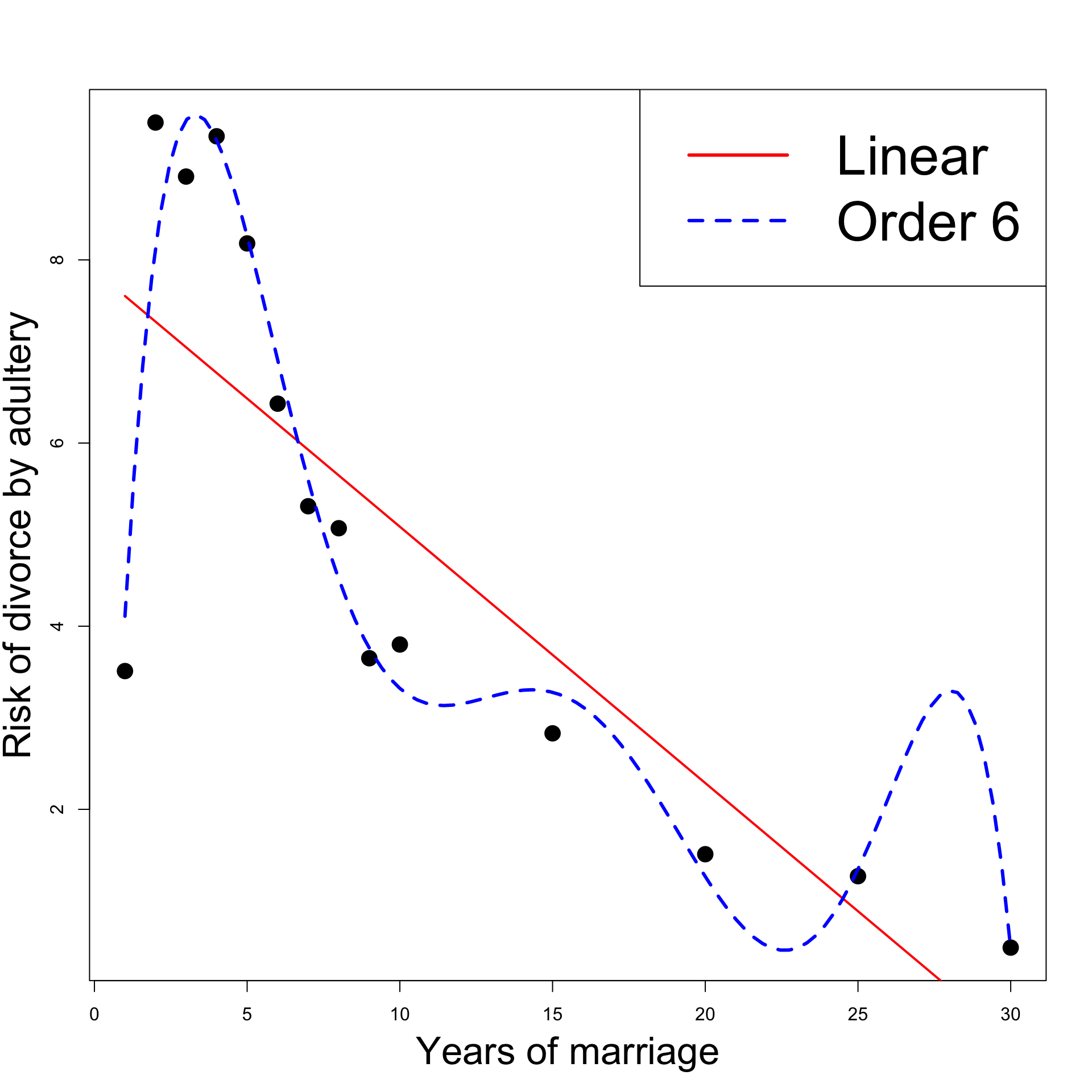

Akaike information criterion (AIC)

• The AIC is a number which measures how well a regression model fits the data

• Also R^2 measures how well a regression model fits the data

• The difference between AIC and R^2 is that AIC also accounts for overfitting

• The formal definition of AIC is

{\rm AIC} := 2p - 2 \log ( \hat{L} )

• p = number of parameters in the model

• \hat{L} = maximum value of the likelihood function

Akaike information criterion (AIC)

• In past lectures we have shown that for the general regression model

\ln(\hat L)= -\frac{n}{2}\ln(2\pi) - \frac{n}{2}\ln(\hat\sigma^2) - \frac{1}{2\hat\sigma^2} \mathop{\mathrm{RSS}}\,, \qquad \hat \sigma^2 := \frac{\mathop{\mathrm{RSS}}}{n}

• Therefore

\ln(\hat L)= - \frac{n}{2} \log \left( \frac{\mathop{\mathrm{RSS}}}{n} \right) + C

• C is constant depending only on the number of sample points

• Thus C does not change if the data does not change

Akaike information criterion (AIC)

• We obtain the following equivalent formula for AIC

{\rm AIC} = 2p + n \log \left( \frac{ \mathop{\mathrm{RSS}}}{n} \right) - 2C

• We now see that AIC accounts for
  • Data fit: since the data fit term \mathop{\mathrm{RSS}} is present
  • Model complexity: Since the number of degrees of freedom p is present
• Therefore a model with low AIC is such that:
  1. Model fits data well
  2. Model is not too complex, preventing overfitting
• Conclusion: sometimes AIC is better than R^2 when comparing two models

Stepwise regression and AIC

• Stepwise regression function in R uses AIC to compare models
  • the model with lowest AIC is selected
• Hence Stepwise regression outputs the model which, at the same time
  1. Best fits the given data
  2. Prevents overfitting
• Example: Apply Stepwise regression to divorces examples to compare
  • Linear model
  • Order 6 model

Example: Divorces

The dataset

• Code for this example is available here divorces_stepwise.R

Years of Marriage	1	2	3	4	5	6	7
% divorces adultery	3.51	9.50	8.91	9.35	8.18	6.43	5.31

Years of Marriage	8	9	10	15	20	25	30
% divorces adultery	5.07	3.65	3.80	2.83	1.51	1.27	0.49

Fitting the null model

• First we import the data into R

# Divorces data
year <- c(1, 2, 3, 4, 5, 6,7, 8, 9, 10, 15, 20, 25, 30)
percent <- c(3.51, 9.5, 8.91, 9.35, 8.18, 6.43, 5.31, 
             5.07, 3.65, 3.8, 2.83, 1.51, 1.27, 0.49)

• The null model is

{\rm percent} = \beta_1 + \varepsilon

• Fit the null model with

null.model <- lm(percent ~ 1)

Fitting the full model

• The full model is the Order 6 model

\rm{percent} = \beta_1 + \beta_2 \, {\rm year} + \beta_3 \, {\rm year}^2 + \ldots + \beta_7 \, {\rm year}^6

• Fit the full model with

full.model <- lm(percent ~ year  + I( year^2 ) + I( year^3 ) + 
                                   I( year^4 ) + I( year^5 ) +
                                   I( year^6 ))

Stepwise regression

• We run stepwise regression and save the best model

best.model <- step(null.model, 
                  direction = "both", 
                  scope = formula(full.model)) 

• The best model is Linear, and not Order 6!

summary(best.model)

Call:
lm(formula = percent ~ year)

.....

Conclusions

• Old conclusions:
  • Linear model has lower R^2 than Order 6 model
  • F-test for model selection chooses Order 6 model over Linear model
  • Hence Order 6 model seems better than Linear model
• New conclusions:
  • Order 6 model is more complex than the Linear model
  • In particular Order 6 model has higher AIC than the Linear model
  • Stepwise regression chooses Linear model over Order 6 model
• Bottom line: The new findings are in line with our intuition:
  • Order 6 model overfits
  • Therefore the Linear model should be preferred

Part 5:
Dummy variable
regression models

Outline

1. Dummy variable regression
2. Factors in R
3. ANOVA models
4. ANOVA F-test and regression
5. Two-way ANOVA
6. Two-way ANOVA with interactions
7. ANCOVA

Part 1:
Dummy variable
regression

Explaining the terminology

• Dummy variable: Variables X which are quantitative in nature

• ANOVA: refers to situations where regression models contain

  • only dummy variables X

• ANCOVA: refers to situations where regression models contain a combination of

  • dummy variables and quantitative (the usual) variables

Dummy variables

• Dummy variable:

  • A variable X which is qualitative in nature
  • Often called cathegorical variables

• Regression models can include dummy variables

• Qualitatitve binary variables can be represented by X with

  • X = 1 \, if effect present
  • X = 0 \, if effect not present

• Examples of binary quantitative variables are

  • On / Off
  • Yes / No
  • Sample is from Population A / B

Dummy variables

• Dummy variables can also take several values
  • These values are often called levels
  • Such variables are represented by X taking discrete values
• Examples of dummy variables with several levels
  • Season: Summer, Autumn, Winter, Spring
  • Sex: Male, Female, Non-binary, …
  • Priority: Low, Medium, High
  • Quarterly sales data: Q1, Q2, Q3, Q4
  • UK regions: East Midlands, London Essex, North East/Yorkshire, …

Example: Fridge sales data

• Consider the dataset on quarterly fridge sales fridge_sales.txt
  • Each entry represents sales data for 1 quarter
  • 4 consecutive entries represent sales data for 1 year

   fridge.sales durable.goods.sales Q1 Q2 Q3 Q4 Quarter
1          1317               252.6  1  0  0  0       1
2          1615               272.4  0  1  0  0       2
3          1662               270.9  0  0  1  0       3
4          1295               273.9  0  0  0  1       4
5          1271               268.9  1  0  0  0       1
6          1555               262.9  0  1  0  0       2
7          1639               270.9  0  0  1  0       3
8          1238               263.4  0  0  0  1       4
9          1277               260.6  1  0  0  0       1
10         1258               231.9  0  1  0  0       2
11         1417               242.7  0  0  1  0       3
12         1185               248.6  0  0  0  1       4
13         1196               258.7  1  0  0  0       1
14         1410               248.4  0  1  0  0       2
15         1417               255.5  0  0  1  0       3
16          919               240.4  0  0  0  1       4
17          943               247.7  1  0  0  0       1
18         1175               249.1  0  1  0  0       2
19         1269               251.8  0  0  1  0       3
20          973               262.0  0  0  0  1       4
21         1102               263.3  1  0  0  0       1
22         1344               280.0  0  1  0  0       2
23         1641               288.5  0  0  1  0       3
24         1225               300.5  0  0  0  1       4
25         1429               312.6  1  0  0  0       1
26         1699               322.5  0  1  0  0       2
27         1749               324.3  0  0  1  0       3
28         1117               333.1  0  0  0  1       4
29         1242               344.8  1  0  0  0       1
30         1684               350.3  0  1  0  0       2
31         1764               369.1  0  0  1  0       3
32         1328               356.4  0  0  0  1       4

• Below are the first 4 entries of the Fridge sales dataset
  • These correspond to 1 year of sales data
• First two variables are quantitative
  • Fridge Sales = total quarterly fridge sales (in million $)
  • Duarable Goods Sales = total quarterly durable goods sales (in billion $)
• Remaining variables are qualitative:
  • Q1, Q2, Q3, Q4 \, take values 0 / 1 \quad (representing 4 yearly quarters)
  • Quarter \, takes values 1 / 2 / 3 / 4 \quad (equivalent representation of quarters)

Fridge Sales	Durable Goods Sales	Q1	Q2	Q3	Q4	Quarter
1317	252.6	1	0	0	0	1
1615	272.4	0	1	0	0	2
1662	270.9	0	0	1	0	3
1295	273.9	0	0	0	1	4

Encoding Quarter in regression model

Two alternative approaches:

1. Include 4-1 = 3 dummy variables with values 0 / 1
   • Each dummy variable represents 1 Quarter
   • We need 3 variables to represent 4 Quarters (if we include intercept)
2. Include one variable which takes values 1 / 2 / 3 / 4

Differences between the two approaches:

1. This method is good to first understand dummy variable regression

2. This is the most efficient way of organising cathegorical data in R

   • usese the command \, \texttt{factor}

The dummy variable trap

• Suppose you follow the first approach:
  • Encode each quarter with a separate variable
• If you have 4 different levels you would need
  • 4-1=3 dummy variables
  • the intercept term
• In general: if you have m different levels you would need
  • m-1 dummy variables
  • the intercept term

Question: Why only m - 1 dummy variables?

Answer: To avoid the dummy variable trap

Example: Dummy variable trap

To illustrate the dummy variable trap consider the following

• Encode each Quarter with one dummy variable D_i

D_i = \begin{cases} 1 & \text{ if data belongs to Quarter i} \\ 0 & \text{ otherwise} \\ \end{cases}

• Consider the regression model with intercept

Y = \beta_0 \cdot (1) + \beta_1 D_1 + \beta_2 D_2 + \beta_3 D_3 + \beta_4 D_4 + \varepsilon

• In the above Y is the quartely Fridge sales data

• Each data entry belongs to exactly one Quarter, so that

D_1 + D_2 + D_3 + D_4 = 1

• Dummy variable trap: Variables are collinear (linearly dependent)

• Indeed the design matrix is

Z = \left( \begin{array}{ccccc} 1 & 1 & 0 & 0 & 0 \\ 1 & 0 & 1 & 0 & 0 \\ 1 & 0 & 0 & 1 & 0 \\ 1 & 0 & 0 & 0 & 1 \\ 1 & 1 & 0 & 0 & 0 \\ \dots & \dots & \dots & \dots & \dots \\ \end{array} \right)

• First column is the sum of remaining columns \quad \implies \quad Multicollinearity

Example: Avoiding dummy variable trap

• We want to avoid Multicollinearity (or dummy variable trap)

• How? Drop one dummy variable (e.g. the first) and consider the model

Y = \beta_1 \cdot (1) + \beta_2 D_2 + \beta_3 D_3 + \beta_4 D_4 + \varepsilon

• If data belongs to Q1 then D_2 = D_3 = D_4 = 0

• Therefore, in general, we have

D_2 + D_3 + D_4 \not\equiv 1

• This way we avoid Multicollinearity \quad \implies \quad no trap!

• Question: How do we interpret the coefficients in the model

Y = \beta_1 \cdot (1) + \beta_2 D_2 + \beta_3 D_3 + \beta_4 D_4 + \varepsilon\qquad ?

• Answer: Recall the relationship

D_1 + D_2 + D_3 + D_4 = 1

• Substituting in the regression model we get

\begin{align*} Y & = \beta_1 \cdot ( D_1 + D_2 + D_3 + D_4 ) + \beta_2 D_2 + \beta_3 D_3 + \beta_4 D_4 + \varepsilon\\[10pts] & = \beta_1 D_1 + (\beta_1 + \beta_2) D_2 + (\beta_1 + \beta_3) D_3 + (\beta_1 + \beta_4 ) D_4 + \varepsilon \end{align*}

• Therefore the regression coefficients are such that
  • \beta_1 describes increase for D_1
  • \beta_1 + \beta_2 describes increase for D_2
  • \beta_1 + \beta_3 describes increase for D_3
  • \beta_1 + \beta_4 describes increase for D_4

Conclusion: When fitting regression model with dummy variables

• Increase for first dummy variable D_1 is intercept term \beta_1

• Increase for successive dummy variables D_i with i > 1 is computed by \beta_1 + \beta_i

Intercept coefficient acts as base reference point

General case: Dummy variable trap

• Suppose to have a qualitative X variable which takes m different levels
  • E.g. the previous example has m = 4 quarters
• Encode each level of X in one dummy variable D_i

D_i = \begin{cases} 1 & \text{ if X has level i} \\ 0 & \text{ otherwise} \\ \end{cases}

• To each data entry corresponds one and only one level of X, so that

D_1 + D_2 + \ldots + D_m = 1

• Hence Multicollinearity if intercept is present \, \implies \, Dummy variable trap!

General case: Avoid the trap!

• We drop the first dummy variable D_1 and consider the model

Y = \beta_1 \cdot (1) + \beta_2 D_2 + \beta_3 D_3 + \ldots + \beta_m D_m + \varepsilon

• For data points such that X = 1 we have

D_2 = D_3 = \ldots = D_m = 0

• Therefore, in general, we get

D_2 + D_3 + \ldots + D_m \not \equiv 1

• This way we avoid Multicollinearity \quad \implies \quad no trap!

General case: Interpret the output

• How to interpret the coefficients in the model

Y = \beta_1 \cdot (1) + \beta_2 D_2 + \beta_3 D_3 + \ldots + \beta_m D_m + \varepsilon\quad ?

• We can argue similarly to the case m = 4 and use the constraint

D_1 + D_2 + \ldots + D_m = 1

• Substituting in the regression model we get

Y = \beta_1 D_1 + (\beta_1 + \beta_2) D_2 + \ldots + (\beta_1 + \beta_m) D_m + \varepsilon

Conclusion: When fitting regression model with dummy variables

• Increase for first dummy variable D_1 is intercept term \beta_1

• Increase for successive dummy variables D_i with i > 1 is computed by \beta_1 + \beta_i

Intercept coefficient acts as base reference point

Part 2:
Factors in R

Factors in R

• Before proceeding we need to introduce factors in R

• Factors: A way to represent discrete variables taking a finite number of values

• Example: Suppose to have a vector of people’s names

firstname <- c("Liz", "Jolene", "Susan", "Boris", "Rochelle", "Tim")

• Let us store the sex of each person as either
  • Numbers: \, \texttt{1} represents female and \texttt{0} represents male
  • Strings: \, \texttt{"female"} and \texttt{"male"}

sex.num <- c(1, 1, 1, 0, 1, 0)
sex.char <- c("female", "female", "female", "male", "female", "male")

The factor command

• The \, \texttt{factor} command turns a vector into a factor

# Turn sex.num into a factor
sex.num.factor <- factor(sex.num)

# Print the factor obtained
print(sex.num.factor)

[1] 1 1 1 0 1 0
Levels: 0 1

• The factor \, \texttt{sex.num.factor} looks like the original vector \, \texttt{sex.num}

• The difference is that the factor \, \texttt{sex.num.factor} contains levels

  • In this case the levels are \, \texttt{0} and \, \texttt{1}
  • Levels are all the (discrete) values assumed by the vector \, \texttt{sex.num}

The factor command

• In the same way we can convert \, \texttt{sex.char} into a factor

# Turn sex.char into a factor
sex.char.factor <- factor(sex.char)

# Print the factor obtained
print(sex.char.factor)

[1] female female female male   female male  
Levels: female male

• Again, the factor \, \texttt{sex.char.factor} looks like the original vector \, \texttt{sex.char}

• Again, the difference is that the factor \, \texttt{sex.char.factor} contains levels

  • In this case the levels are strings \, \texttt{"female"} and \, \texttt{"male"}
  • These 2 strings are all the values assumed by the vector \, \texttt{sex.char}

Subsetting factors

• Factors can be subset exactly like vectors

sex.num.factor[2:5]

[1] 1 1 0 1
Levels: 0 1

Subsetting factors

• Warning: After subsetting a factor, all defined levels are still stored
  • This is true even if some of the levels are no longer represented in the subsetted factor

subset.factor <- sex.char.factor[c(1:3, 5)]

print(subset.factor)

[1] female female female female
Levels: female male

• The levels of \, \texttt{subset.factor} are still \, \texttt{"female"} and \, \texttt{"male"}

• This is despite \, \texttt{subset.factor} only containing \, \texttt{"female"}

The levels function

• The levels of a factor can be extracted with the function \, \texttt{levels}

levels(sex.char.factor)

[1] "0" "1"

• Note: Levels of a factor are always stored as strings, even if originally numbers

levels(sex.num.factor)

[1] "0" "1"

• The levels of \, \texttt{sex.num.factor} are the strings \, \texttt{"0"} and \, \texttt{"1"}

• This is despite the original vector \, \texttt{sex.num} being numeric

• The command \, \texttt{factor} converted numeric levels into strings

Relabelling a factor

• The function \, \texttt{levels} can also be used to relabel factors

• For example we can relabel

  • \, \texttt{female} into \, \texttt{f}
  • \, \texttt{male} into \, \texttt{m}

# Relabel levels of sex.char.factor
levels(sex.char.factor) <- c("f", "m")

# Print relabelled factor
print(sex.char.factor)

[1] f f f m f m
Levels: f m

Logical subsetting of factors

• Logical subsetting is done exactly like in the case of vectors

• Important: Need to remember that levels are always strings

• Example: To identify all the men in \, \texttt{sex.num.factor} we do

sex.num.factor == "0"

[1] FALSE FALSE FALSE  TRUE FALSE  TRUE

• To retrieve names of men stored in \, \texttt{firstname} use logical subsetting

firstname[ sex.num.factor == "0" ]

[1] "Boris" "Tim"  

Part 3:
ANOVA models

Analysis of variance (ANOVA) models in R

• The data in fridge_sales.txt links
  • Sales of fridges and Sales of durable goods
  • to the time of year (Quarter)
• For the moment ignore the data on the Sales of durable goods

• Goal: Fit regression and analysis of variance models to link
  • Fridge sales to the time of the year

• There are two ways this can be achieved in R
  1. A regression approach using the command \, \texttt{lm}
  2. An analysis of variance (ANOVA) approach using the command \, \texttt{aov}

• Code for this example is available here anova.R

• Data is in the file fridge_sales.txt

• The first 4 rows of the data-set are given below

  fridge.sales durable.goods.sales Q1 Q2 Q3 Q4 Quarter
1         1317               252.6  1  0  0  0       1
2         1615               272.4  0  1  0  0       2
3         1662               270.9  0  0  1  0       3
4         1295               273.9  0  0  0  1       4

• Therefore we have the variables
  • Fridge sales
  • Durable goods sales \quad (ignored for now)
  • Q1, Q2, Q3, Q4
  • Quarter

Reading the data into R

• We read the data into a data-frame as usual

# Load dataset on Fridge Sales
sales <- read.table(file = "fridge_sales.txt",
                    header = TRUE)

# Assign data-frame columns to vectors
fridge <- sales[ , 1]
durables <- sales[ , 2]
q1 <- sales[ , 3]
q2 <- sales[ , 4]
q3 <- sales[ , 5]
q4 <- sales[ , 6]
quarter <- sales[ , 7]

Processing dummy variables in R

• The variables \, \texttt{q1, q2, q3, q4} \, are vectors taking the values \, \texttt{0} and \, \texttt{1}
  • No further data processing is needed for \, \texttt{q1, q2, q3, q4}
  • Remember: To avoid dummy variable trap only 3 of these 4 dummy variables can be included (if the model also includes an intercept term)

• The variable \, \texttt{quarter} is a vector taking the values \, \texttt{1}, \texttt{2}, \texttt{3}, \texttt{4}
  • Need to tell R this is a qualitative variable
  • This is done with the \, \texttt{factor} command

factor(quarter)

 [1] 1 2 3 4 1 2 3 4 1 2 3 4 1 2 3 4 1 2 3 4 1 2 3 4 1 2 3 4 1 2 3 4
Levels: 1 2 3 4

Regression and ANOVA

As already mentioned, there are 2 ways of fitting regression and ANOVA models in R

1. A regression approach using the command \, \texttt{lm}
2. An analysis of variance approach using the command \, \texttt{aov}

• Both approaches lead to the same numerical answers in our example

Regression approach

We can proceed in 2 equivalent ways

1. Use a dummy variable approach (and arbitrarily excluding \, \texttt{q1})

# We drop q1 to avoid dummy variable trap
dummy.lm <- lm (fridge ~ q2 + q3 + q4)
summary(dummy.lm)

2. Using the \, \texttt{factor} command on \, \texttt{quarter}

# Need to convert quarter to a factor
quarter.f <- factor(quarter)

factor.lm <- lm(fridge ~ quarter.f)
summary(factor.lm)

• Get the same numerical answers using both approaches

Output for dummy variable approach

Call:
lm(formula = fridge ~ q2 + q3 + q4)

Coefficients:
            Estimate Std. Error t value Pr(>|t|)    
(Intercept)  1222.12      59.99  20.372  < 2e-16 ***
q2            245.37      84.84   2.892 0.007320 ** 
q3            347.63      84.84   4.097 0.000323 ***
q4            -62.12      84.84  -0.732 0.470091    
---
Signif. codes:  0 ‘***’ 0.001 ‘**’ 0.01 ‘*’ 0.05 ‘.’ 0.1 ‘ ’ 1

Residual standard error: 169.7 on 28 degrees of freedom
Multiple R-squared:  0.5318,    Adjusted R-squared:  0.4816 
F-statistic:  10.6 on 3 and 28 DF,  p-value: 7.908e-05

Output for factor approach

Call:
lm(formula = fridge ~ quarter.f)

Coefficients:
            Estimate Std. Error t value Pr(>|t|)    
(Intercept)  1222.12      59.99  20.372  < 2e-16 ***
quarter.f2    245.37      84.84   2.892 0.007320 ** 
quarter.f3    347.63      84.84   4.097 0.000323 ***
quarter.f4    -62.12      84.84  -0.732 0.470091    
---
Signif. codes:  0 ‘***’ 0.001 ‘**’ 0.01 ‘*’ 0.05 ‘.’ 0.1 ‘ ’ 1

Residual standard error: 169.7 on 28 degrees of freedom
Multiple R-squared:  0.5318,    Adjusted R-squared:  0.4816 
F-statistic:  10.6 on 3 and 28 DF,  p-value: 7.908e-05

• The two outputs are essentially the same (only difference is variables names)

• \, \texttt{quarter.f} is a factor with four levels \, \texttt{1}, \texttt{2}, \texttt{3}, \texttt{4}

• Variables \, \texttt{quarter.f2}, \texttt{quarter.f3}, \texttt{quarter.f4} refer to the levels \, \texttt{2}, \texttt{3}, \texttt{4} in \, \texttt{quarter.f}

Output for factor approach

Call:
lm(formula = fridge ~ quarter.f)

Coefficients:
            Estimate Std. Error t value Pr(>|t|)    
(Intercept)  1222.12      59.99  20.372  < 2e-16 ***
quarter.f2    245.37      84.84   2.892 0.007320 ** 
quarter.f3    347.63      84.84   4.097 0.000323 ***
quarter.f4    -62.12      84.84  -0.732 0.470091    
---
Signif. codes:  0 ‘***’ 0.001 ‘**’ 0.01 ‘*’ 0.05 ‘.’ 0.1 ‘ ’ 1

Residual standard error: 169.7 on 28 degrees of freedom
Multiple R-squared:  0.5318,    Adjusted R-squared:  0.4816 
F-statistic:  10.6 on 3 and 28 DF,  p-value: 7.908e-05

• \, \texttt{lm} is treating \, \texttt{quarter.f2}, \texttt{quarter.f3}, \texttt{quarter.f4} as if they were dummy variables

• Note that \, \texttt{lm} automatically drops \, \texttt{quarter.f1} to prevent dummy variable trap

• Thus \, \texttt{lm} behaves the same way as if we passed dummy variables \, \texttt{q2}, \texttt{q3}, \texttt{q4}

Computing regression coefficients

Call:
lm(formula = fridge ~ q2 + q3 + q4)

Coefficients:
            Estimate Std. Error t value Pr(>|t|)    
(Intercept)  1222.12      59.99  20.372  < 2e-16 ***
q2            245.37      84.84   2.892 0.007320 ** 
q3            347.63      84.84   4.097 0.000323 ***
q4            -62.12      84.84  -0.732 0.470091    

• Recall that \, \texttt{Intercept} refers to coefficient for \, \texttt{q1}

• Coefficients for \, \texttt{q2}, \texttt{q3}, \texttt{q4} are obtained by summing \, \texttt{Intercept} to coefficient in appropriate row

Computing regression coefficients

Call:
lm(formula = fridge ~ q2 + q3 + q4)

Coefficients:
            Estimate Std. Error t value Pr(>|t|)    
(Intercept)  1222.12      59.99  20.372  < 2e-16 ***
q2            245.37      84.84   2.892 0.007320 ** 
q3            347.63      84.84   4.097 0.000323 ***
q4            -62.12      84.84  -0.732 0.470091    

Dummy variable	Coefficient formula	Estimated coefficient
\texttt{q1}	\beta_1	1222.12
\texttt{q2}	\beta_1 + \beta_2	1222.12 + 245.37 = 1467.49
\texttt{q3}	\beta_1 + \beta_3	1222.12 + 347.63 = 1569.75
\texttt{q4}	\beta_1 + \beta_4	1222.12 - 62.12 = 1160

Regression formula

• Therefore the linear regression formula obtained is

\begin{align*} {\rm I\kern-.3em E}[\text{ Fridge sales } ] = & \,\, 1222.12 \times \, \text{Q1} + 1467.49 \times \, \text{Q2} + \\[15pts] & \,\, 1569.75 \times \, \text{Q3} + 1160 \times \, \text{Q4} \end{align*}

• Recall that Q1, Q2, Q3 and Q4 assume only values 0 / 1 and

\text{Q1} + \text{Q2} + \text{Q4} + \text{Q4} = 1

Sales estimates

Therefore the expected sales for each quarter are

\begin{align*} {\rm I\kern-.3em E}[\text{ Fridge sales } | \text{ Q1 } = 1] & = 1222.12 \\[15pts] {\rm I\kern-.3em E}[\text{ Fridge sales } | \text{ Q2 } = 1] & = 1467.49 \\[15pts] {\rm I\kern-.3em E}[\text{ Fridge sales } | \text{ Q3 } = 1] & = 1569.75 \\[15pts] {\rm I\kern-.3em E}[\text{ Fridge sales } | \text{ Q4 } = 1] & = 1160 \\[15pts] \end{align*}

ANOVA for the same problem

• First of all: What is ANOVA?

• ANOVA stands for Analysis of Variance

• ANOVA is used to compare means of independent populations:

  • Suppose to have M normally distributed populations N(\mu_k, \sigma^2) \,\,\,\,\qquad (with same variance)
  • The goal is to compare the populations averages \mu_k
  • For M = 2 this can be done with the two-sample t-test
  • For M > 2 we use ANOVA

ANOVA is a generalization of two-sample t-test to multiple populations

The ANOVA F-test

• To compare populations averages we use the hypotheses

\begin{align*} H_0 & \colon \mu_{1} = \mu_{2} = \ldots = \mu_{M} \\ H_1 & \colon \mu_i \neq \mu_j \, \text{ for at least one pair i and j} \end{align*}

• To decide on the above hypothesis we use the ANOVA F-test

• We omit mathematical details. All you need to know is that

  • ANOVA F-test is performed in R with the function \, \texttt{aov}
  • This function outputs the so-called ANOVA table
  • ANOVA table contains the F-statistic and relative p-value for ANOVA F-test

If p < 0.05 we reject H_0 and there is a difference in populations averages

ANOVA F-test for fridge sales

• In the Fridge Sales example we wish to compare Fridge sales numbers
  • We have Fridge Sales data for each quarter
  • Each Quarter represents a population
  • We want to compare average fridge sales for each Quarter

• ANOVA hypothesis test: is there a difference in average sales for each Quarter?
  • If \mu_{i} is average sales in Quarter i then \begin{align*} H_0 & \colon \mu_{1} = \mu_{2} = \mu_{3} = \mu_{4} \\ H_1 & \colon \mu_i \neq \mu_j \, \text{ for at least one pair i and j} \end{align*}

Plotting the data

• Plot Quarter against Fridge sales

plot(quarter, fridge)

• We clearly see 4 populations

• Averages appear different

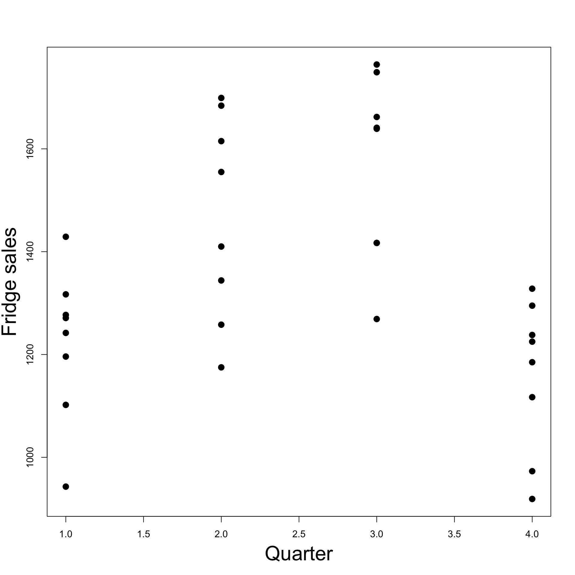
ANOVA F-test for fridge sales

• To implement ANOVA F-test in R you need to use command \, \texttt{factor}

# Turn vector quarter into a factor
quarter.f <- factor(quarter)

• The factor \, \texttt{quarter.f} \, allows to label the fridge sales data
  • Factor level \, \texttt{k} \, corresponds to fridge sales in Quarter k

• To perform the ANOVA F-test do

# Fit ANOVA model
factor.aov <- aov(fridge ~ quarter.f)

# Print output
summary(factor.aov)

ANOVA output

• The summary gives the following analysis of variance (ANOVA) table

            Df Sum Sq Mean Sq F value   Pr(>F)    
quarter.f    3 915636  305212    10.6 7.91e-05 ***
Residuals   28 806142   28791                     
---
Signif. codes:  0 ‘***’ 0.001 ‘**’ 0.01 ‘*’ 0.05 ‘.’ 0.1 ‘ ’ 1

• The F-statistic for the ANOVA F-test is \,\, F = 10.6

• The p-value for ANOVA F-test is \,\, p = 7.91 \times 10^{-5}

• Therefore p < 0.05 and we reject H_0

  • Evidence that average Fridge sales are different in at least two quarters

ANOVA F-statistic from regression

Alternative way to get ANOVA F-statistic: Look at output of dummy variable model

\texttt{lm(fridge} \, \sim \, \texttt{q2 + q3 + q4)}

Residual standard error: 169.7 on 28 degrees of freedom
Multiple R-squared:  0.5318,    Adjusted R-squared:  0.4816 
F-statistic:  10.6 on 3 and 28 DF,  p-value: 7.908e-05

• The F-test for overall fit gives
  • F-statistic \,\, F = 10.6
  • p-value \,\, p = 7.908 \times 10^{-5}

These always coincide with F-statistic and p-value for ANOVA F-test! \quad Why?

Part 5:
ANOVA F-test
and regression

ANOVA F-test and regression

• ANOVA F-test equivalent to F-test for overall significance

• This happens because
  • Linear regression can be used to perform ANOVA F-test

• We have already seen a particular instance of this fact in the Homework
  • Simple linear regression can be used to perform two-sample t-test

• This was done by considering the model

Y_i = \alpha + \beta \, 1_B (i) + \varepsilon_i

Simple regression for two-sample t-test

In more details:

• A and B are two normal populations N(\mu_A, \sigma^2) and N(\mu_B, \sigma^2)

• We have two samples

  • Sample of size n_A from population A a = (a_1, \ldots, a_{n_A})
  • Sample of size n_B from population B b = (b_1, \ldots, b_{n_B})

Simple regression for two-sample t-test

• The data vector y is obtained by concatenating a and b

y = (a,b) = (a_1, \ldots, a_{n_A}, b_1, \ldots, b_{n_B} )

• We then considered the dummy variable model

Y_i = \alpha + \beta \, 1_B (i) + \varepsilon_i

• Here 1_B (i) is the dummy variable relative to population B

1_B(i) = \begin{cases} 1 & \text{ if i-th sample belongs to population B} \\ 0 & \text{ otherwise} \end{cases}

Simple regression for two-sample t-test

• The regression function is therefore

{\rm I\kern-.3em E}[Y | 1_B = x] = \alpha + \beta x

• By construction we have that

Y | \text{sample belongs to population A} \ \sim \ N(\mu_A, \sigma^2)

• Therefore by definition of 1_B we get

{\rm I\kern-.3em E}[Y | 1_B = 0] = {\rm I\kern-.3em E}[Y | \text{ sample belongs to population A}] = \mu_A

Simple regression for two-sample t-test

• On the other hand, the regression function is

{\rm I\kern-.3em E}[Y | 1_B = x] = \alpha + \beta x

• Thus

{\rm I\kern-.3em E}[Y | 1_B = 0] = \alpha + \beta \cdot 0 = \alpha

• Recall that \, {\rm I\kern-.3em E}[Y | 1_B = 0] = \mu_A

• Hence we get

\alpha = \mu_A

Simple regression for two-sample t-test

• Similarly, we get that

{\rm I\kern-.3em E}[Y | 1_B = 1] = {\rm I\kern-.3em E}[Y | \text{ sample belongs to population B}] = \mu_B

• On the other hand, using the regression function we get

{\rm I\kern-.3em E}[Y | 1_B = 1] = \alpha + \beta \cdot 1 = \alpha + \beta

• Therefore

\alpha + \beta = \mu_B

Simple regression for two-sample t-test

• Since \alpha = \mu_A we get

\alpha + \beta = \mu_B \quad \implies \quad \beta = \mu_B - \mu_A

• In particular we have shown that the regression model is

\begin{align*} Y_i & = \alpha + \beta \, 1_{B} (i) + \varepsilon_i \\[10pts] & = \mu_A + (\mu_B - \mu_A) \, 1_{B} (i) + \varepsilon_i \end{align*}

Simple regression for two-sample t-test

• F-test for overall significance for previous slide model is

\begin{align*} H_0 \colon \beta = 0 \\ H_1 \colon \beta \neq 0 \end{align*}

• Since \beta = \mu_B - \mu_A the above is equivalent to

\begin{align*} H_0 \colon \mu_A = \mu_B \\ H_1 \colon \mu_A \neq \mu_B \end{align*}

F-test for overall significance is equivalent to two-sample t-test

ANOVA F-test and regression

We now consider the general ANOVA case

• Suppose to have M populations A_i with normal distribution N(\mu_i,\sigma^2) \qquad (with same variance)

• Example: In Fridge sales example we have M = 4 populations (the 4 quarters)

• The ANOVA F-test for difference in populations means is

\begin{align*} H_0 & \colon \mu_1 = \mu_2 = \ldots = \mu_M \\ H_1 & \colon \mu_i \neq \mu_j \text{ for at least one pair i and j} \end{align*}

• Goal: Show that the above test can be obtained with regression

Setting up dummy variable model

• We want to introduce dummy variable regression model which models ANOVA

• To each population A_i associate a dummy variable

1_{A_i}(i) = \begin{cases} 1 & \text{ if i-th sample belongs to population } A_i \\ 0 & \text{ otherwise} \\ \end{cases}

• Suppose to have samples a_i of size n_{A_i} from population A_i

• Concatenate these samples into a long vector (length n_{A_1} + \ldots + n_{A_M})

y = (a_1, \ldots, a_M)

Setting up dummy variable model

• Consider the dummy variable model (with 1_{A_1} omitted)

Y_i = \beta_1 + \beta_2 \, 1_{A_2} (i) + \beta_3 \, 1_{A_3} (i) + \ldots + \beta_M \, 1_{A_M} (i) + \varepsilon_i

• The regression function is therefore

{\rm I\kern-.3em E}[Y | 1_{A_2} = x_2 , \, \ldots, \, 1_{A_M} = x_M ] = \beta_1 + \beta_2 \, x_2 + \ldots + \beta_M \, x_M

• By construction we have that

Y | \text{sample belongs to population } A_i \ \sim \ N(\mu_i , \sigma^2)

Conditional expectations

• The sample belongs to population A_1 if and only if

1_{A_2} = 1_{A_3} = \ldots = 1_{A_M} = 0

• Hence we can compute the conditional expectation

{\rm I\kern-.3em E}[ Y | 1_{A_2} = 0 , \, \ldots, \, 1_{A_M} = 0] = {\rm I\kern-.3em E}[Y | \text{sample belongs to population } A_1] = \mu_1

• On the other hand, by definition of regression function, we get

{\rm I\kern-.3em E}[ Y | 1_{A_2} = 0 , \, \ldots, \, 1_{A_M} = 0] = \beta_1 + \beta_2 \cdot 0 + \ldots + \beta_M \cdot 0 = \beta_1

• We conclude that \,\, \mu_1 = \beta_1

Conditional expectations

• Similarly, the sample belongs to population A_2 if and only if

1_{A_2} = 1 \quad \text{and} \quad 1_{A_1} = 1_{A_3} = \ldots = 1_{A_M} = 0

• Hence we can compute the conditional expectation

{\rm I\kern-.3em E}[ Y | 1_{A_2} = 1 , \, \ldots, \, 1_{A_M} = 0] = {\rm I\kern-.3em E}[Y | \text{sample belongs to population } A_2] = \mu_2

• On the other hand, by definition of regression function, we get

{\rm I\kern-.3em E}[ Y | 1_{A_2} = 1 , \, \ldots, \, 1_{A_M} = 0] = \beta_1 + \beta_2 \cdot 1 + \ldots + \beta_M \cdot 0 = \beta_1 + \beta_2

• We conclude that \,\, \mu_2 = \beta_1 + \beta_2

Conditional expectations

• We have shown that

\mu_1 = \beta_1 \quad \text{ and } \quad \mu_2 = \beta_1 + \beta_2

• Therefore we obtain

\beta_1 = \mu_1 \quad \text{ and } \quad \beta_2 = \mu_2 - \mu_1

• Arguing in a similar way, we can show that also

\beta_i = \mu_i - \mu_1 \qquad \forall \, i > 1

Conclusion

• The considered dummy variable model is

\begin{align*} Y_i & = \beta_1 + \beta_2 \, 1_{A_2} (i) + \ldots + \beta_M \, 1_{A_M} (i) + \varepsilon_i \end{align*}

• The F-test of overall significance for the above regression model is

\begin{align*} H_0 & \colon \beta_2 = \beta_3 = \ldots = \beta_M = 0 \\ H_1 & \colon \text{ At least one of the above } \beta_j \neq 0 \end{align*}

• We have also shown that

\beta_1 = \mu_1 \,, \qquad \beta_i = \mu_i - \mu_1 \quad \forall \, i > 1

• In particular we obtain

\begin{align*} \beta_2 = \ldots = \beta_M = 0 & \quad \iff \quad \mu_2 - \mu_1 = \ldots = \mu_M - \mu_1 = 0 \\[10pts] & \quad \iff \quad \mu_2 = \ldots = \mu_M = \mu_1 \end{align*}

• Thefore the F-test for overall significance is equivalent to ANOVA F-test

\begin{align*} H_0 & \colon \mu_1 = \mu_2 = \ldots = \mu_M \\ H_1 & \colon \mu_i \neq \mu_j \text{ for at least one pair i and j} \end{align*}

F-test for overall significance is equivalent to ANOVA F-test

References

[1]

Gujarati, D. N., Porter, D. C., Basic econometric, fifth edition, McGraw-Hill, 2009.

[2]

Draper, N. R., Smith, H., Applied regression analysis, Wiley, 1998.

[3]

Shumway, R. H., Stoffer, D. S., Time series analysis and its applications, fourth edition, Springer, 2017.