Part 3:
Basic question in regression
What happens to Y as X increases?
increases?
decreases?
nothing?
Positive gradient
As X increases Y increases
Negative gradient
As X increases Y decreases
Zero gradient
Changes in X do not affect Y
t-test for simple regression
Consider the simple linear regression model
Y_i = \alpha + \beta X_i + \varepsilon_i
X \,\, \text{ affects } \,\, Y \qquad \iff \qquad
\beta \neq 0
\begin{align*}
H_0 \colon & \beta = b \\
H_1 \colon & \beta \neq b
\end{align*}
Construction of t-test
\begin{align*}
H_0 \colon & \beta = b \\
H_1 \colon & \beta \neq b
\end{align*}
Distribution of \hat \beta
Theorem Consider the linear regression model
Y_i = \alpha + \beta x_i + \varepsilon_i
with \varepsilon_i iid N(0, \sigma^2) . Then
\hat \beta \sim N \left(\beta , \frac{ \sigma^2 }{ S_{xx} } \right)
Proof: Quite difficult. If interested see Theorem 11.3.3 in [1 ]
Construction of the t-statistic
We want to construct t-statistic for \hat \beta
As for the standard t-test, we want a t-statistic of the form
t = \frac{\text{Estimate } - \text{ Hypothesised Value}}{\mathop{\mathrm{e.s.e.}}}
\hat \beta \sim N \left(\beta , \frac{ \sigma^2 }{ S_{xx} } \right)
Construction of the t-statistic
In particular \hat \beta is an unbiased estimator for \beta
{\rm I\kern-.3em E}[ \hat \beta ] = \beta
Therefore \hat \beta is the estimate
t = \frac{\text{Estimate } - \text{ Hypothesised Value}}{\mathop{\mathrm{e.s.e.}}}
= \frac{ \hat \beta - \beta }{ \mathop{\mathrm{e.s.e.}}}
Estimated Standard Error
{\rm Var}[\hat \beta] = \frac{ \sigma^2 }{ S_{xx}}
Hence the standard error of \hat \beta is the standard deviation
{\rm SD}[\hat \beta] = \frac{ \sigma }{ S_{xx} }
{\rm SD} cannot be used for testing, since \sigma^2 is unknown
Estimated Standard Error
We however have an estimate for \sigma^2
\hat \sigma^2 = \frac{1}{n} \mathop{\mathrm{RSS}}= \frac1n \sum_{i=1}^n (y_i - \hat y_i)^2
{\rm I\kern-.3em E}[ \hat\sigma^2 ] = \frac{n-2}{n} \, \sigma^2
Estimated Standard Error
S^2 := \frac{n}{n-2} \, \hat\sigma^2 = \frac{\mathop{\mathrm{RSS}}}{n-2}
This way S^2 is unbiased estimator for \sigma^2
{\rm I\kern-.3em E}[S^2] = \frac{n}{n-2} \, {\rm I\kern-.3em E}[\hat\sigma^2] = \frac{n}{n-2} \, \frac{n-2}{n} \, \sigma^2 = \sigma^2
Estimated Standard Error
Recall that the standard deviation of \hat \beta is
{\rm SD}[\hat \beta] = \frac{ \sigma }{ S_{xx} }
\mathop{\mathrm{e.s.e.}}= \frac{S}{\sqrt{S_{xx}}}
t-statistic to test \hat \beta
The t-statistic for \hat \beta is then
t = \frac{\text{Estimate } - \text{ Hypothesised Value}}{\mathop{\mathrm{e.s.e.}}}
= \frac{ \hat \beta - \beta }{ S / \sqrt{S_{xx}} }
Theorem Consider the linear regression model
Y_i = \alpha + \beta x_i + \varepsilon_i
with \varepsilon_i iid N(0, \sigma^2) . Then
t = \frac{ \hat \beta - \beta }{ S / \sqrt{S_{xx}} }
\, \sim \,
t_{n-2}
How to prove the Theorem
Proof of this Theorem is quite difficult and we omit it
If you are interested in the proof, see Section 11.3.4 in [1 ]
The main idea is that t-statistic can be rewritten as
t = \frac{ \hat \beta - \beta }{ S / \sqrt{S_{xx}} }
= \frac{ U }{ \sqrt{ V/(n-2) } }
U := \frac{ \hat \beta - \beta }{ \sigma / \sqrt{S_{xx}} } \,, \qquad \quad V := \frac{ (n-2) S^2 }{ \sigma^2 }
How to prove the Theorem
\hat \beta \sim N \left(\beta , \frac{ \sigma^2 }{ S_{xx} } \right)
U = \frac{ \hat \beta - \beta }{ \sigma / \sqrt{S_{xx}} } \, \sim \, N(0,1)
How to prove the Theorem
Moreover it can be shown that
V = \frac{(n-2) S^2}{\sigma^2} \, \sim \, \chi_{n-2}^2
It can also be shown that U and V are independent
How to prove the Theorem
t = \frac{ \hat \beta - \beta }{ S / \sqrt{S_{xx}} }
= \frac{ U }{ \sqrt{ V/(n-2) } }
U and V are independent, with
U \sim N(0,1) \,, \qquad \quad V \sim \chi_{n-2}^2
From the Theorem on t-distribution in Lecture 3 we conclude
t \sim t_{n-2}
Summary: t-test for \beta
Goal : Estimate the slope \beta for the simple linear model
Y_i = \alpha + \beta x_i + \varepsilon_i \,, \qquad \varepsilon_i \, \text{ iid } \, N(0,\sigma^2)
Hypotheses : If b is guess for \beta the hypotheses are
\begin{align*}
H_0 & \colon \beta = b \\
H_1 & \colon \beta \neq b
\end{align*}
Summary: t-test for \beta
t = \frac{\hat \beta - b }{ \mathop{\mathrm{e.s.e.}}} \, \sim \, t_{n-2} \,, \qquad \quad
\mathop{\mathrm{e.s.e.}}= \frac{S }{\sqrt{S_{xx}} }
\hat \beta = \frac{ S_{xy} }{ S_{xx} } \,, \qquad \quad S^2 := \frac{\mathop{\mathrm{RSS}}}{n-2}
p = 2 P( t_{n-2} > |t| )
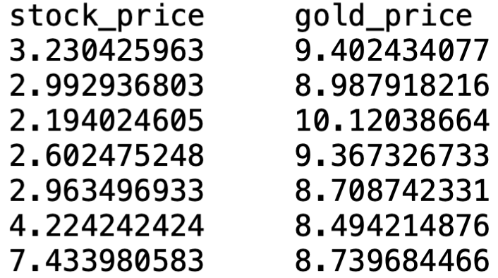
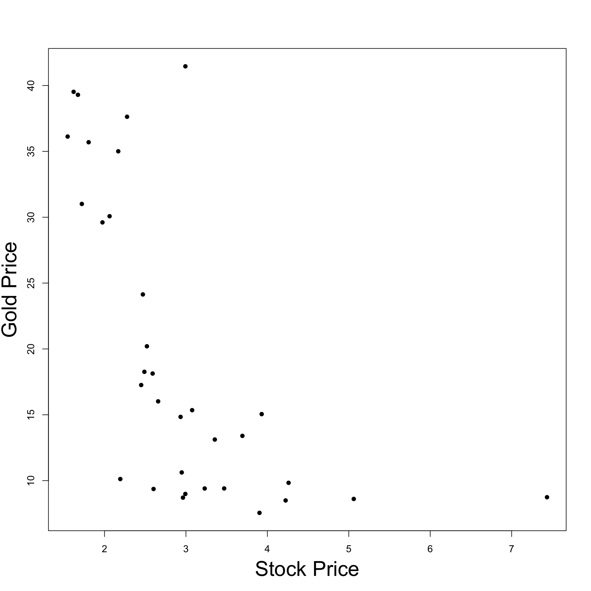
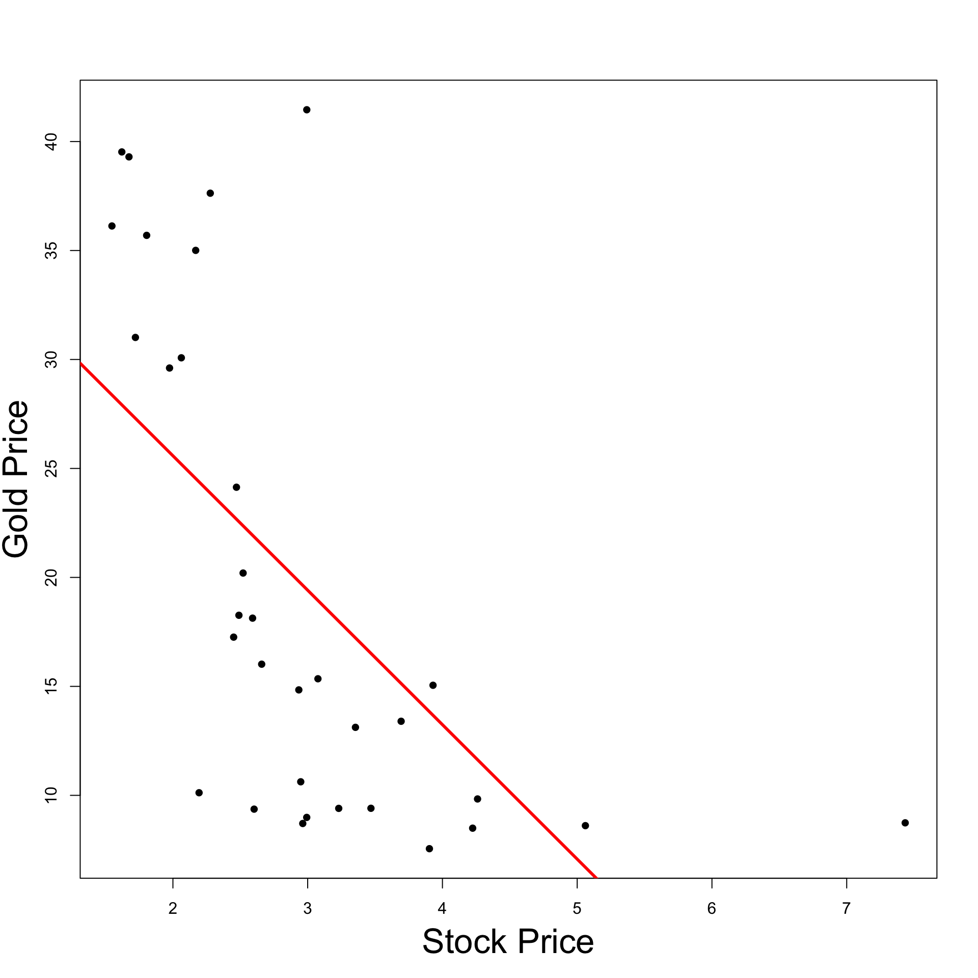
Example: Stock and Gold prices
Recall that
Y = Gold PriceX = Stock Price
We want to test if Gold Price affects Stock Price at level 0.05
Consider the linear model
Y_i = \alpha + \beta x_i + \varepsilon_i
Test the hypotheses \begin{align*}
H_0 & \colon \beta = 0 \\
H_1 & \colon \beta \neq 0
\end{align*}
Testing for \beta = 0
Recall that Stock Prices and Gold Prices are stored in R vectors
Fit the simple linear model with the following commands
\text{gold.price } = \alpha + \beta \, \times \text{ stock.price } + \text{ error}
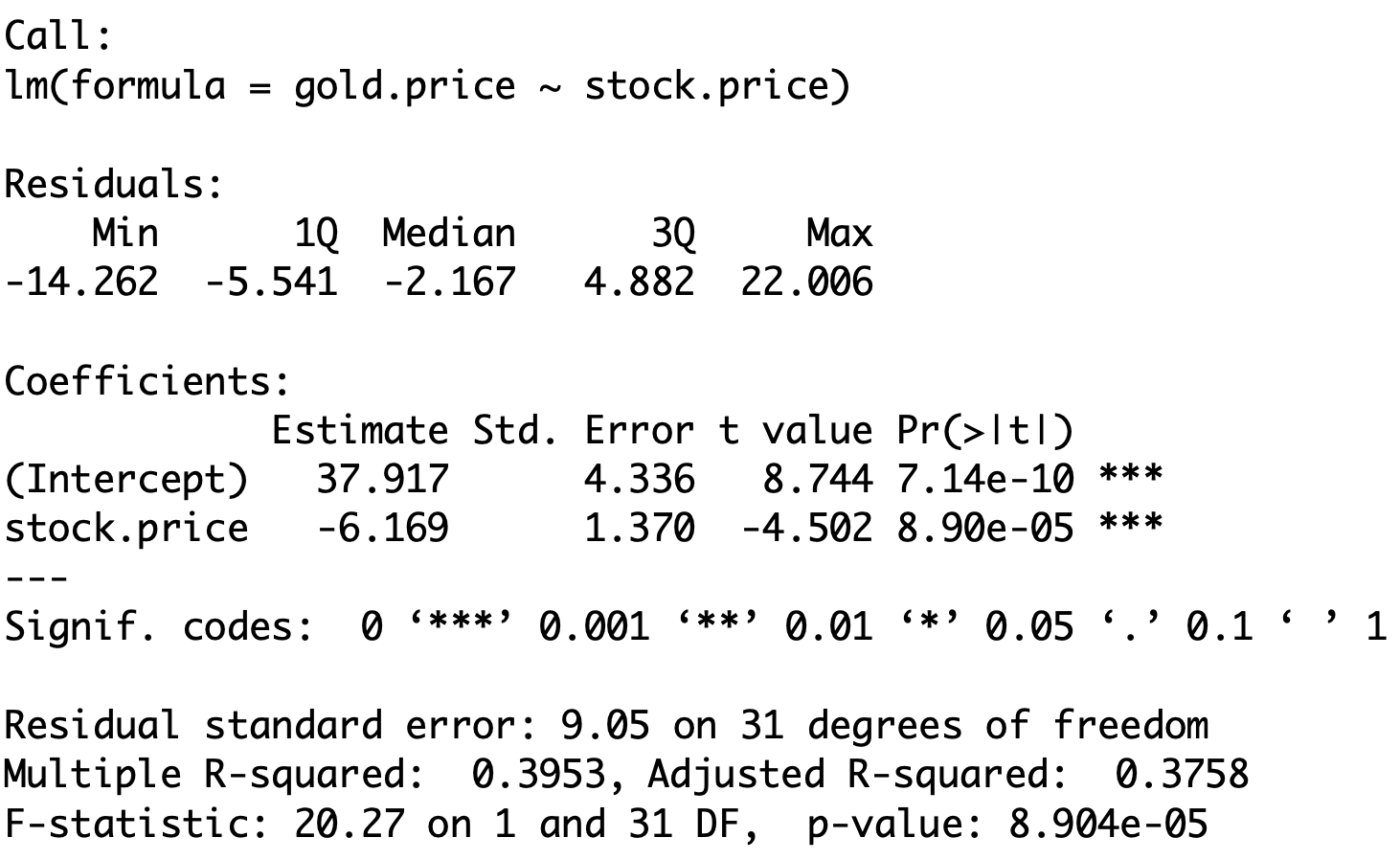
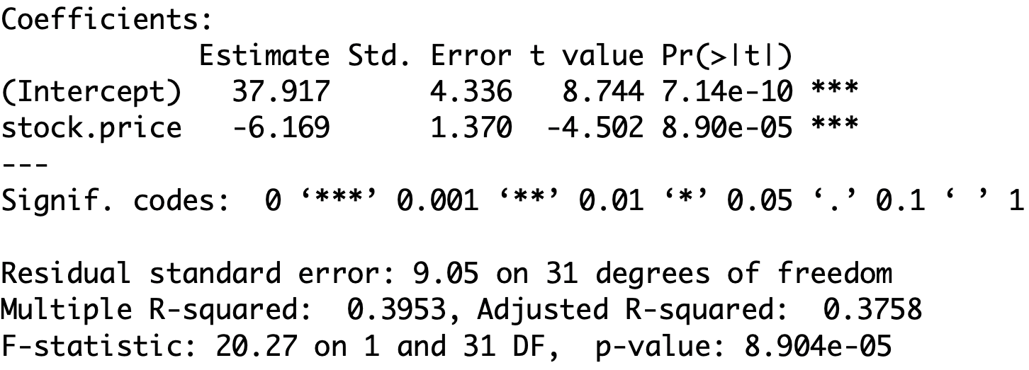
# Fit simple linear regression model <- lm (gold.price ~ stock.price)# Print result to screen summary (fit.model)
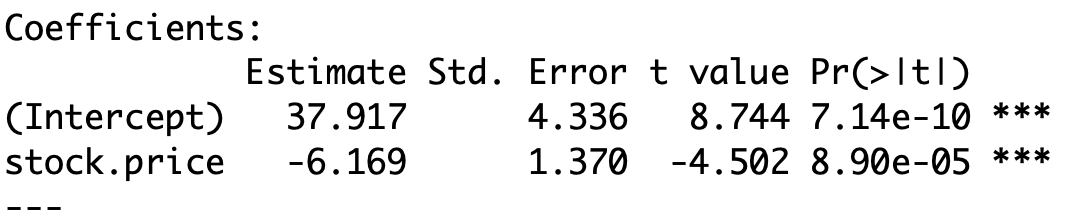
Output: \mathop{\mathrm{e.s.e.}} , t-statistic, p-value
Output: \mathop{\mathrm{e.s.e.}} , t-statistic, p-value
The 2nd row of the table has to be interpreted as follows
\texttt{Std. Error} Estimated standard error \mathop{\mathrm{e.s.e.}} for \beta
\texttt{t value} t-statistic \, t = \dfrac{\hat \beta - 0 }{\mathop{\mathrm{e.s.e.}}}
\texttt{Pr(>|t|)} p-value \, p = 2 P( t_{n-2} > |t| )
\texttt{*} , \, \texttt{**} , \, \texttt{***} , \, \texttt{.} Statistical significance – More stars is better
Output: \mathop{\mathrm{e.s.e.}} , t-statistic, p-value
The above table then gives
\hat \beta = -6.169 \,, \qquad \mathop{\mathrm{e.s.e.}}= 1.37 \, , \qquad t = - 4.502 \,, \qquad
p = 8.9 \times 10^{-5} \
The t -statistic computed by R can also be computed by hand
t = \frac{\hat \beta - 0}{ \mathop{\mathrm{e.s.e.}}}
= \frac{-6.169}{1.37} = -4.502
Output: \mathop{\mathrm{e.s.e.}} , t-statistic, p-value
n = \text{No. of data points} = 33 \,, \qquad \text{df} = n - 2 = 31
Critical value is \, t_{31}(0.025) = 2.040
|t| = 4.502 > 2.040 = t_{31}(0.025) \quad \implies \quad p < 0.05
Output: \mathop{\mathrm{e.s.e.}} , t-statistic, p-value
Interpretation: \, p is very small (hence the \, \texttt{***} \, rating)
Therefore we reject the null hypothesis H_0 and the real parameter is \beta \neq 0
Since \beta \neq 0 we have that Stock Prices affect Gold Prices
The best estimate for \beta is \hat \beta = -6.169
\hat \beta < 0 and statistically significant:\,\, As Stock Prices increase Gold Prices decrease
t-test for general regression
Consider the general linear regression model
Y_i = \beta_1 z_{i1} + \ldots + \beta_{ip} z_{ip} + \varepsilon_i \,, \qquad
\varepsilon_i \, \text{ iid } \, N(0, \sigma^2)
Z_j \,\, \text{ affects } \,\, Y \qquad \iff \qquad
\beta_j \neq 0
To see if Z_j affects Y we need to test the hypothesis
\begin{align*}
H_0 \colon & \beta_j = b_j \\
H_1 \colon & \beta_j \neq b_j
\end{align*}
Distribution of estimator \hat \beta
The estimator for the general model is
\hat \beta = (Z^T Z)^{-1} Z^T y
It can be proven that (see Section 11.5 in [2 ] )
\hat \beta_j \sim N \left( \beta_j , \xi_{jj} \sigma^2 \right)
The numbers \xi_{jj} are the diagonal entries of the p \times p matrix
(Z^T Z)^{-1} =
\left(
\begin{array}{ccc}
\xi_{11} & \ldots & \xi_{1p} \\
\ldots & \ldots & \ldots \\
\xi_{p1} & \ldots & \xi_{pp} \\
\end{array}
\right)
Construction of the t-statistic
In particular \hat \beta_j is an unbiased estimator for \beta_j
{\rm I\kern-.3em E}[ \hat \beta_j ] = \beta_j
Therefore the t-statistic for \hat \beta_j is
t = \frac{\text{Estimate } - \text{ Hypothesised Value}}{\mathop{\mathrm{e.s.e.}}}
= \frac{ \hat \beta_j - \beta_j }{ \mathop{\mathrm{e.s.e.}}}
Estimated Standard Error
{\rm Var}[\hat \beta_j] = \xi_{jj} \, \sigma^2
Hence the standard error of \hat \beta_j is the standard deviation
{\rm SD}[\hat \beta_j] = \xi_{jj}^{1/2} \, \sigma
{\rm SD} cannot be used for testing, since \sigma^2 is unknown
Estimated Standard Error
We however have an estimate for \sigma^2
\hat \sigma^2 = \frac{1}{n} \mathop{\mathrm{RSS}}= \frac1n \sum_{i=1}^n (y_i - \hat y_i)^2
{\rm I\kern-.3em E}[ \hat\sigma^2 ] = \frac{n-p}{n} \, \sigma^2
Estimated Standard Error
S^2 := \frac{n}{n-p} \, \hat\sigma^2 = \frac{\mathop{\mathrm{RSS}}}{n-p}
This way S^2 is unbiased estimator for \sigma^2
{\rm I\kern-.3em E}[S^2] = \frac{n}{n-p} \, {\rm I\kern-.3em E}[\hat\sigma^2] = \frac{n}{n-p} \, \frac{n-p}{n} \, \sigma^2 = \sigma^2
Estimated Standard Error
Recall that the standard deviation of \hat \beta is
{\rm SD}[\hat \beta] = \xi_{jj}^{1/2} \, \sigma
\mathop{\mathrm{e.s.e.}}=\xi_{jj}^{1/2} \, S
t-statistic to test \beta_j
Theorem Consider the general linear regression model
Y_i = \beta_1 z_{i1} + \ldots +\beta_p z_{ip} + \varepsilon_i
with \varepsilon_i iid N(0, \sigma^2) . Then
t = \frac{\text{Estimate } - \text{ Hypothesised Value}}{\mathop{\mathrm{e.s.e.}}} = \frac{ \hat \beta_j - \beta_j }{ \xi_{jj}^{1/2} \, S}
\, \sim \,
t_{n-p}
Proof: See section 11.5 in [2 ]
Summary: t-test for \beta_j
Goal : Estimate the coefficient \beta_j for the general linear model
Y_i = \beta_1 z_{i1} + \ldots + \beta_p z_{ip} + \varepsilon_i \,, \qquad \varepsilon_i \, \text{ iid } \, N(0,\sigma^2)
Hypotheses : If b_j is guess for \beta_j the hypotheses are
\begin{align*}
H_0 & \colon \beta_j = b_j \\
H_1 & \colon \beta_j \neq b_j
\end{align*}
Summary: t-test for \beta_j
t = \frac{\hat \beta_j - b_j }{ \mathop{\mathrm{e.s.e.}}} \, \sim \, t_{n-p} \,, \qquad \quad
\mathop{\mathrm{e.s.e.}}= \xi_{jj}^{1/2} \, S
In the above \xi_{jj} are diagonal entries of (Z^TZ)^{-1} and
\hat \beta = (Z^TZ)^{-1} Z^T y \,, \qquad \quad S^2 := \frac{\mathop{\mathrm{RSS}}}{n-p}
p = 2P (t_{n-p} > |t|)
t-test in R: Fit general regression with lm
If b_j = 0 and a two-sided t-test is required
t-statistic is in j -th variable row under \,\, \texttt{t value}
p-value is in j -th variable row under \,\, \texttt{Pr(>|t|)}
If b_j \neq 0 or one-sided t-test is required
Compute t-statistic by hand
t = \frac{\hat \beta_j - b_j}{\mathop{\mathrm{e.s.e.}}}
\,\, \hat \beta_j is in j -th variable row under \,\, \texttt{Estimate} \,\, \mathop{\mathrm{e.s.e.}} for \hat \beta_j is in j -th variable row under \,\, \texttt{Std. Error} Compute p-value by hand with \,\, \texttt{pt(t, df)}
Example: \mathop{\mathrm{e.s.e.}} for simple linear regression
Consider the simple regression model
Y_i = \alpha + \beta x_i + \varepsilon_i
Z = \left(
\begin{array}{cc}
1 & x_1 \\
\ldots & \ldots \\
1 & x_n \\
\end{array}
\right)
Example: \mathop{\mathrm{e.s.e.}} for simple linear regression
We have seen in Lecture 9 that
(Z^T Z)^{-1} =
\frac{1}{n S_{xx} }
\left(
\begin{array}{cc}
\sum_{i=1}^n x^2_i & -n \overline{x}\\
-n\overline{x} & n
\end{array}
\right)
Hence the \mathop{\mathrm{e.s.e.}} for \hat \alpha and \hat \beta are
\begin{align*}
\mathop{\mathrm{e.s.e.}}(\hat \alpha) & = \xi_{11}^{1/2} \, S^2 = \sqrt{ \frac{ \sum_{i=1}^n x_i^2 }{ n S_{xx} } } \, S^2 \\[7pt]
\mathop{\mathrm{e.s.e.}}(\hat \beta) & = \xi_{22}^{1/2} \, S^2 = \frac{ S^2 }{ \sqrt{ S_{xx} } }
\end{align*}
Note: \, \mathop{\mathrm{e.s.e.}}(\hat\beta) coincides with the \mathop{\mathrm{e.s.e.}} in Slide 50
Part 4:
F-test for overall significance
Want to test the overall significance of the model
Y_i = \beta_1 + \beta_2 x_{i2} + \ldots + \beta_p x_{ip} + \varepsilon_i
This means answering the question:
\text{ Does at least one } X_i \text{ affect } Y \text{ ?}
How to do this?
Could perform a sequence of t-tests on the \beta_j
For statistical reasons this is not really desirable
To assess overall significance we can perform F-test
F-test for overall significance
The F-test for overall significance has 3 steps:
Define a larger full model (with more parameters)
Define a smaller nested reduced model (with fewer parameters)
Use an F-statistic to decide between larger or smaller model
Overall significance for multiple regression
Model 1 is the smaller reduced model
Model 2 is the larger full model
\begin{align*}
\textbf{Model 1:} & \quad Y_i = \beta_1 + \varepsilon_i \\[15pt]
\textbf{Model 2:} & \quad Y_i = \beta_1 + \beta_2 x_{i2} + \ldots + \beta_p x_{ip} + \varepsilon_i
\end{align*}
Choosing the smaller Model 1 is equivalent to accepting H_0
\begin{align*}
H_0 & \colon \, \beta_2 = \beta_3 = \ldots = \beta_p = 0 \\
H_1 & \colon \text{ At least one of the } \beta_i \text{ is non-zero}
\end{align*}
Overall significance for simple regression
Model 1 is the smaller reduced model
Model 2 is the larger full model
\begin{align*}
\textbf{Model 1:} & \quad Y_i = \alpha + \varepsilon_i \\[15pt]
\textbf{Model 2:} & \quad Y_i = \alpha + \beta x_i + \varepsilon_i
\end{align*}
Choosing the smaller Model 1 is equivalent to accepting H_0
\begin{align*}
H_0 & \colon \beta = 0 \\
H_1 & \colon \beta \neq 0
\end{align*}
Construction of F-statistic
Consider the full model with p parameters
\textbf{Model 2:} \quad Y_i = \beta_1 + \beta_2 x_{i2} + \ldots + \beta_p x_{ip} + \varepsilon_i
Predictions for the full model are
\hat y_i := \beta_1 + \beta_2 x_{i2} + \ldots + \beta_p x_{ip}
Define the residual sum of squares for the full model
\mathop{\mathrm{RSS}}(p) := \sum_{i=1}^n (y_i - \hat y_i)^2
Construction of F-statistic
Consider now the reduced model
\textbf{Model 1:} \quad Y_i = \beta_1 + \varepsilon_i
Predictions of the reduced model are constant
\hat y_i = \beta_1
Define the residual sum of squares for the full model
\mathop{\mathrm{RSS}}(1) := \sum_{i=1}^n (y_i - \beta_1)^2
Construction of F-statistic
Suppose the parameters of the full model
\beta_2, \ldots, \beta_p
are not important
In this case the predictions of full and reduced model will be similar
Therefore the \mathop{\mathrm{RSS}} for the 2 models are similar
\mathop{\mathrm{RSS}}(1) \, \approx \, \mathop{\mathrm{RSS}}(p)
Construction of F-statistic
Recall that \mathop{\mathrm{RSS}} is defined via minimization
\mathop{\mathrm{RSS}}(k) := \min_{\beta_1 , \ldots , \beta_k} \ \sum_{i=1}^n ( y_i - \hat y_i)^2 \,, \qquad
\hat y_i := \beta_1 + \beta_2 x_{i2} + \ldots + \beta_k x_{ik}
Therefore \mathop{\mathrm{RSS}} cannot increase if we add parameters to the model
\mathop{\mathrm{RSS}}(1) \geq \mathop{\mathrm{RSS}}(p)
To measure how influential the parameters \beta_2, \ldots, \beta_p are, we study
\frac{\mathop{\mathrm{RSS}}(1) - \mathop{\mathrm{RSS}}(p)}{\mathop{\mathrm{RSS}}(p)}
Construction of F-statistic
\frac{\mathop{\mathrm{RSS}}(1) - \mathop{\mathrm{RSS}}(p)}{\mathop{\mathrm{RSS}}(p)}
To this end, note that the degrees of freedom of reduced model are
\mathop{\mathrm{df}}(1) = n - 1
The degrees of freedom of the full model are
\mathop{\mathrm{df}}(p) = n - p
F-statistic for overall significance
Definition The
F-statistic for overall significance is
\begin{align*}
F & := \frac{\mathop{\mathrm{RSS}}(1) - \mathop{\mathrm{RSS}}(p)}{ \mathop{\mathrm{df}}(1) - \mathop{\mathrm{df}}(p) } \bigg/
\frac{\mathop{\mathrm{RSS}}(p)}{\mathop{\mathrm{df}}(p)} \\[15pt]
& = \frac{\mathop{\mathrm{RSS}}(1) - \mathop{\mathrm{RSS}}(p)}{ p - 1 } \bigg/
\frac{\mathop{\mathrm{RSS}}(p)}{n - p}
\end{align*}
Theorem: The F-statistic for overall significance has F-distribution
F \, \sim \, F_{p-1,n-p}
Rewriting the F-statistic
Proposition The F-statistic can be rewritten as
\begin{align*}
F & = \frac{\mathop{\mathrm{RSS}}(1) - \mathop{\mathrm{RSS}}(p)}{ p - 1 } \bigg/
\frac{\mathop{\mathrm{RSS}}(p)}{n - p} \\[15pt]
& = \frac{R^2}{1 - R^2} \, \cdot \, \frac{n - p}{p - 1}
\end{align*}
Proof of Proposition
Notice that \mathop{\mathrm{TSS}} does not depend on p since
\mathop{\mathrm{TSS}}= \sum_{i=1}^n (y_i - \overline{y})^2
Recall the definition of R^2
R^2 = 1 - \frac{\mathop{\mathrm{RSS}}(p)}{\mathop{\mathrm{TSS}}}
\mathop{\mathrm{RSS}}(p) = (1 - R^2) \mathop{\mathrm{TSS}}
Proof of Proposition
By definition we have that
\mathop{\mathrm{RSS}}(1) = \min_{\beta_1} \ \sum_{i=1}^n (y_i - \beta_1)^2
Exercise: Check that the unique solution to the above problem is
\beta_1 = \overline{y}
\mathop{\mathrm{RSS}}(1) = \sum_{i=1}^n (y_i - \overline{y})^2 = \mathop{\mathrm{TSS}}
Proof of Proposition
We just obtained the two identities
\mathop{\mathrm{RSS}}(p) = (1 - R^2) \mathop{\mathrm{TSS}}\,, \qquad \quad \mathop{\mathrm{RSS}}(1) = \mathop{\mathrm{TSS}}
From the above we conclude the proof
\begin{align*}
F & = \frac{\mathop{\mathrm{RSS}}(1) - \mathop{\mathrm{RSS}}(p)}{ p - 1 } \bigg/
\frac{\mathop{\mathrm{RSS}}(p)}{n - p} \\[15pt]
& = \frac{\mathop{\mathrm{TSS}}- (1 - R^2) \mathop{\mathrm{TSS}}}{ p - 1 } \bigg/
\frac{(1 - R^2) \mathop{\mathrm{TSS}}}{n - p}\\[15pt]
& = \frac{R^2}{1 - R^2} \, \cdot \, \frac{n - p}{p - 1}
\end{align*}
F-statistic for simple regression
Proposition
The F -statistic for overall significance in simple regression is
F = t^2 \,, \qquad \quad t = \frac{\hat \beta}{ S / \sqrt{S_{xx}}}
where t is the t-statistic for \hat \beta .
In particular the p-values for t-test and F-test coincide
p = P( t_{n-2} > |t| ) = P( F_{1,n-2} > F )
Proof: Will be left as an exercise
Summary: F-test for overall significance
Goal: Test the overall significance of the model
Y_i = \beta_1 + \beta_2 x_{i2} + \ldots + \beta_p x_{ip} + \varepsilon_i
This means answering the question:
\text{ Does at least one } X_i \text{ affect } Y \text{ ?}
Hypotheses: The above question is equivalent to testing
\begin{align*}
H_0 & \colon \, \beta_2 = \beta_3 = \ldots = \beta_p = 0 \\
H_1 & \colon \text{ At least one of the } \beta_i \text{ is non-zero}
\end{align*}
Summary: F-test for overall significance
\begin{align*}
F & = \frac{\mathop{\mathrm{RSS}}(1) - \mathop{\mathrm{RSS}}(p)}{ p - 1 } \bigg/
\frac{\mathop{\mathrm{RSS}}(p)}{n - p} \\[15pt]
& = \frac{R^2}{1 - R^2} \, \cdot \, \frac{n - p}{p - 1}
\end{align*}
F \, \sim \, F_{p-1,n-p}
Summary: F-test for overall significance
p = P ( F_{p-1,n-2} > F)
F-test in R:
Fit the multiple regression model with lm
F-statistic is listed in the summary
p-value is listed in the summary
Example: Stock and Gold prices
Recall that
Y = Gold PriceX = Stock Price We want to test the overall significance of the model
Y_i = \alpha + \beta x_i + \varepsilon_i
To this end, perform F-test for the hypotheses
\begin{align*}
H_0 & \colon \beta = 0 \\
H_1 & \colon \beta \neq 0
\end{align*}
F-test for overall significance
Recall that Stock Prices and Gold Prices are stored in R vectors
Fit the simple linear model with the following commands
\text{gold.price } = \alpha + \beta \, \times \text{ stock.price } + \text{ error}
# Fit simple linear regression model <- lm (gold.price ~ stock.price)# Print result to screen summary (fit.model)
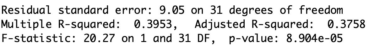
Output: F-statistic and p-value
F-statistic is F = 20.27
Degrees of freedom are 1 and 31 , meaning that F \, \sim \, F_{1,31}
The p-value is
p = P( F_{1,31} > F ) = 8.904 \times 10^{-5}
Conclusion: Strong evidence (p=0.000 ) that Stock Price affects Gold Price
Output: F-statistic and p-value
We can also compute F-statistic by hand
F = \frac{ R^2 }{ 1 - R^2 } \, \cdot \, \frac{n-p}{p-1} = \frac{0.395325}{0.604675} \, \cdot \, \frac{31}{1} = 20.267
Output: F-statistic and p-value
The p-value cannot be computed by hand
However we can find critical values close to F_{1,31} (0.05) on Tables
F_{1, 30} (0.05) = 4.17 \,, \qquad \quad F_{1, 40} (0.05) = 4.08
Output: F-statistic and p-value
We can approximate F_{1,31} (0.05) by averaging the found values
F_{1,31}(0.05) \, \approx \, \frac{F_{1, 30} (0.05) + F_{1, 40} (0.05)}{2} = 4.125
F = 20.267 > 4.125 = F_{1,31}(0.05) \quad \implies \quad p < 0.05
Testing regression parameters
Summary: We have seen
t-test
Test the significance of individual parameters \begin{align*}
H_0 & \colon \, \beta_j = 0 \\
H_1 & \colon \, \beta_j \neq 0
\end{align*}
Testing regression parameters
F-test
Test the overall significance of the model
This is done by comparing two nested regression models \begin{align*}
\textbf{Model 1:} & \qquad Y_ i= \beta_1 + \varepsilon_i \\[10pt]
\textbf{Model 2:} & \qquad Y_ i= \beta_1 + \beta_2 x_{2, i}+ \ldots + \beta_p x_{p, i} + \varepsilon_i
\end{align*}
The comparison is achieved with F-test for \begin{align*}
H_0 & \colon \, \beta_2 = \beta_3 = \ldots = \beta_p = 0 \\
H_1 & \colon \text{ At least one of the } \beta_i \text{ is non-zero}
\end{align*}
Choosing Model 1 is equivalent to accepting H_0
More general nested models
Consider the more general nested models
\begin{align*}
\textbf{Model 1:} & \quad Y_ i =\beta_1 + \beta_2 x_{2, i}+ \ldots + \beta_{k} x_{k, i} + \varepsilon_i \\[10pt]
\textbf{Model 2:} & \quad Y_ i= \beta_1 + \beta_2 x_{2, i}+ \ldots + \beta_{k} x_{k, i} + \beta_{k + 1} x_{k + 1, i} +
\ldots + \beta_{p} x_{p, i} + \varepsilon_i
\end{align*}
\beta_{k + 1} = \beta_{k + 2} = \ldots = \beta_p = 0
Question: How do we decide which model is better?
Model selection
Consider the more general nested models
\begin{align*}
\textbf{Model 1:} & \quad Y_ i =\beta_1 + \beta_2 x_{2, i}+ \ldots + \beta_{k} x_{k, i} + \varepsilon_i \\[10pt]
\textbf{Model 2:} & \quad Y_ i= \beta_1 + \beta_2 x_{2, i}+ \ldots + \beta_{k} x_{k, i} + \beta_{k + 1} x_{k + 1, i} +
\ldots + \beta_{p} x_{p, i} + \varepsilon_i
\end{align*}
Define the predictions for the two models
\begin{align*}
\hat y_i^1 & := \beta_1 + \beta_2 x_{2, i}+ \ldots + \beta_{k} x_{k, i} \\[10pt]
\hat y_i^2 & := \beta_1 + \beta_2 x_{2, i}+ \ldots + \beta_{k} x_{k, i} + \beta_{k + 1} x_{k + 1, i} +
\ldots + \beta_{p} x_{p, i}
\end{align*}
Model selection
Consider the more general nested models
\begin{align*}
\textbf{Model 1:} & \quad Y_ i =\beta_1 + \beta_2 x_{2, i}+ \ldots + \beta_{k} x_{k, i} + \varepsilon_i \\[10pt]
\textbf{Model 2:} & \quad Y_ i= \beta_1 + \beta_2 x_{2, i}+ \ldots + \beta_{k} x_{k, i} + \beta_{k + 1} x_{k + 1, i} +
\ldots + \beta_{p} x_{p, i} + \varepsilon_i
\end{align*}
\mathop{\mathrm{RSS}} measures variation between data and prediction
\begin{align*}
\textbf{Model 1:} & \quad \mathop{\mathrm{RSS}}_1 := \mathop{\mathrm{RSS}}(k) = \sum_{i=1}^n (y_i - \hat y_i^1)^2 \\[10pt]
\textbf{Model 2:} & \quad \mathop{\mathrm{RSS}}_2 := \mathop{\mathrm{RSS}}(p) = \sum_{i=1}^n (y_i - \hat y_i^2)^2
\end{align*}
Construction of F-statistic
Goal: Use \mathop{\mathrm{RSS}} to construct statistic to compare the 2 models
Suppose the extra parameters of Model 2
\beta_{k+1}, \, \beta_{k+2} , \, \ldots , \, \beta_p
are not important
Hence the predictions of the 2 models will be similar
\hat y_i^1 \, \approx \, \hat y_i^2
Therefore the \mathop{\mathrm{RSS}} for the 2 models are similar
\mathop{\mathrm{RSS}}_1 \, \approx \, \mathop{\mathrm{RSS}}_2
Construction of F-statistic
Recall that \mathop{\mathrm{RSS}} cannot increase if we increase parameters
k < p \quad \implies \quad \mathop{\mathrm{RSS}}(k) \geq \mathop{\mathrm{RSS}}(p)
To measure influence of extra parameters
\beta_{k+1}, \, \beta_{k+2} , \, \ldots , \, \beta_p
we consider the ratio
\frac{ \mathop{\mathrm{RSS}}_1 - \mathop{\mathrm{RSS}}_2 }{ \mathop{\mathrm{RSS}}_2 } = \frac{ \mathop{\mathrm{RSS}}(k) - \mathop{\mathrm{RSS}}(p) }{ \mathop{\mathrm{RSS}}(p) }
Construction of F-statistic
\frac{ \mathop{\mathrm{RSS}}_1 - \mathop{\mathrm{RSS}}_2 }{ \mathop{\mathrm{RSS}}_2 }
Note that the degrees of freedom are
Model 1:
k \text{ parameters } \quad \implies \quad \mathop{\mathrm{df}}_1 = n - k
Model 2:
p \text{ parameters } \quad \implies \quad \mathop{\mathrm{df}}_2 = n - p
F-statistic for model selection
Definition The F-statistic for model selection is
\begin{align*}
F & = \frac{ \mathop{\mathrm{RSS}}_1 - \mathop{\mathrm{RSS}}_2 }{ \mathop{\mathrm{df}}_1 - \mathop{\mathrm{df}}_2 } \bigg/
\frac{ \mathop{\mathrm{RSS}}_2 }{ \mathop{\mathrm{df}}_2 } \\[20pt]
& = \frac{ \mathop{\mathrm{RSS}}(k) - \mathop{\mathrm{RSS}}(p) }{ p - k } \bigg/
\frac{ \mathop{\mathrm{RSS}}(p) }{ n - p }
\end{align*}
Theorem: The F-statistic for model selection has F-distribution
F \, \sim \, F_{\mathop{\mathrm{df}}_1 - \mathop{\mathrm{df}}_2 , \, \mathop{\mathrm{df}}_2} = F_{p - k, \, n - p}
Rewriting the F-statistic
Recall the formulas for sums of squares
\mathop{\mathrm{TSS}}= \mathop{\mathrm{ESS}}(p) + \mathop{\mathrm{RSS}}(p) \,, \qquad \quad
\mathop{\mathrm{TSS}}= \mathop{\mathrm{ESS}}(k) + \mathop{\mathrm{RSS}}(k)
R_1^2 := R^2 (k) := \frac{ \mathop{\mathrm{ESS}}(k) }{ \mathop{\mathrm{TSS}}}
\, , \qquad \quad
R_2^2 := R^2 (p) := \frac{ \mathop{\mathrm{ESS}}(p) }{ \mathop{\mathrm{TSS}}}
Rewriting the F-statistic
\begin{align*}
\mathop{\mathrm{RSS}}(k) - \mathop{\mathrm{RSS}}(p) & = \mathop{\mathrm{ESS}}(p) - \mathop{\mathrm{ESS}}(k) \\[10pt]
& = \mathop{\mathrm{TSS}}( R^2(p) - R^2(k) ) \\[10pt]
& = \mathop{\mathrm{TSS}}( R^2_2 - R^2_1 ) \\[20pt]
\mathop{\mathrm{RSS}}(p) & = \mathop{\mathrm{TSS}}- \mathop{\mathrm{ESS}}(p) \\[10pt]
& = \mathop{\mathrm{TSS}}- \mathop{\mathrm{TSS}}\, \cdot \, R^2 (p) \\[10pt]
& = \mathop{\mathrm{TSS}}(1 - R^2(p)) \\[10pt]
& = \mathop{\mathrm{TSS}}(1 - R_2^2)
\end{align*}
Rewriting the F-statistic
Therefore the F-statistic can be rewritten as
\begin{align*}
F & = \frac{ \mathop{\mathrm{RSS}}_1 - \mathop{\mathrm{RSS}}_2 }{ \mathop{\mathrm{df}}_1 - \mathop{\mathrm{df}}_2 } \bigg/
\frac{ \mathop{\mathrm{RSS}}_2 }{ \mathop{\mathrm{df}}_2 } \\[20pt]
& = \frac{ \mathop{\mathrm{TSS}}(R^2_2 - R^2_1) }{\mathop{\mathrm{TSS}}(1 - R^2_2 )} \, \cdot \, \frac{n-p}{p-k} \\[20pt]
& = \frac{ R^2_2 - R^2_1 }{1 - R^2_2} \, \cdot \, \frac{n-p}{p-k}
\end{align*}
F-test for overall significance revisited
The F-test for overall significance allows to select between models \begin{align*}
\textbf{Model 1:} & \qquad Y_ i= \beta_1 + \varepsilon_i \\[10pt]
\textbf{Model 2:} & \qquad Y_ i= \beta_1 + \beta_2 x_{2, i}+ \ldots + \beta_p x_{p, i} + \varepsilon_i
\end{align*}
Model 1 has k = 1 parameters
F-statistic for model selection coincides with F-statistic for overall significance
F = \frac{ \mathop{\mathrm{RSS}}(1) - \mathop{\mathrm{RSS}}(p) }{ p - 1 } \bigg/
\frac{ \mathop{\mathrm{RSS}}(p) }{ n - p }
Summary: F-test for model selection
Goal: Choose one of the nested models
\begin{align*}
\textbf{Model 1:} & \quad Y_ i =\beta_1 + \beta_2 x_{2, i}+ \ldots + \beta_{k} x_{k, i} + \varepsilon_i \\[10pt]
\textbf{Model 2:} & \quad Y_ i= \beta_1 + \beta_2 x_{2, i}+ \ldots + \beta_{k} x_{k, i} + \beta_{k + 1} x_{k + 1, i} +
\ldots + \beta_{p} x_{p, i} + \varepsilon_i
\end{align*}
Hypotheses: Choosing a model is equivalent to testing
\begin{align*}
H_0 \colon & \, \beta_{k+1} = \beta_{k+2} = \ldots = \beta_p \\[5pt]
H_1 \colon & \, \text{ At least one among } \beta_{k+1}, \ldots, \beta_p \text{ is non-zero}
\end{align*}
H_0 is in favor of Model 1H_1 is in favor of Model 2
Summary: F-test for model selection
\begin{align*}
F & = \frac{ \mathop{\mathrm{RSS}}_1 - \mathop{\mathrm{RSS}}_2 }{ \mathop{\mathrm{df}}_1 - \mathop{\mathrm{df}}_2 } \bigg/
\frac{ \mathop{\mathrm{RSS}}_2 }{ \mathop{\mathrm{df}}_2 } \\[20pt]
& = \frac{ R^2_2 - R^2_1 }{1 - R^2_2 } \, \cdot \, \frac{n-p}{p-k}
\end{align*}
F \, \sim \, F_{ \mathop{\mathrm{df}}_1 - \mathop{\mathrm{df}}_2 , \, \mathop{\mathrm{df}}_2 } = F_{p-k, \, n-p}
Summary: F-test for model selection
p = P(F_{p-k,n-p} > F)
F-test for model selection in R:
Fit the two models with \,\texttt{lm}
Use the command \, \texttt{anova} \qquad\quad (more on this later)
Alternative:
Find R^2_1 and R^2_2 in summary
Compute F-statistic and p-value
Part 7:
Examples of model selection
We illustrate F-test for Model Selection with 3 examples:
Joint significance in Multiple linear Regression
Polynomial regression 1
Polynomial regression 2
Example 1: Multiple linear regression
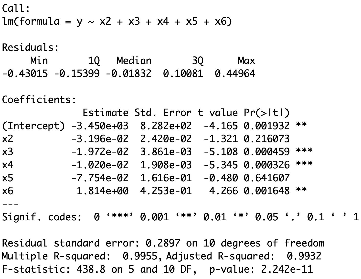
Consider again the Longley dataset
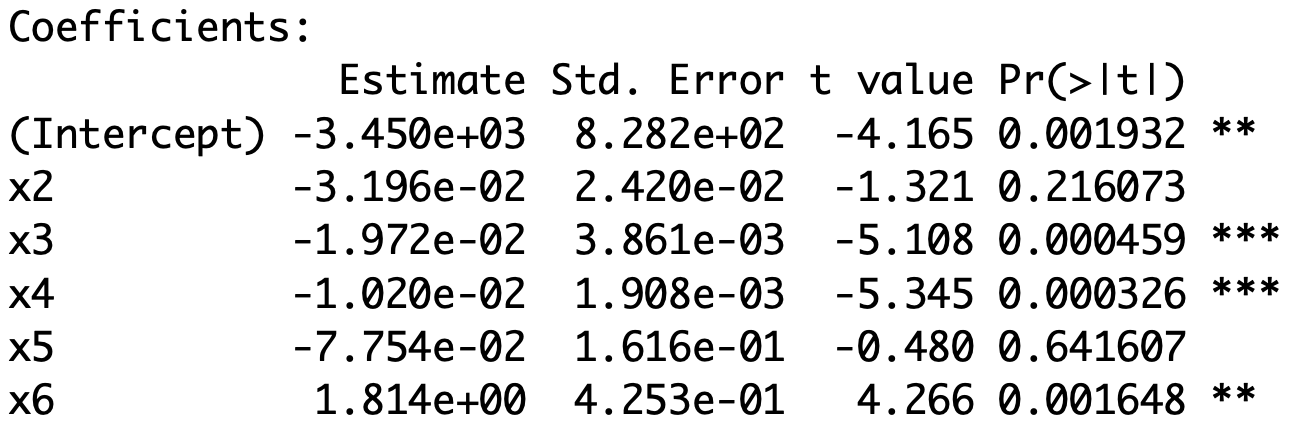
      GNP Unemployed Armed.Forces Population Year Employed
1 234.289      235.6        159.0    107.608 1947   60.323
2 259.426      232.5        145.6    108.632 1948   61.122
3 258.054      368.2        161.6    109.773 1949   60.171
Goal: Explain the number of Employed people Y in the US in terms of
X_2 GNP Gross National ProductX_3 number of Unemployed X_4 number of people in the Armed Forces X_5 non-institutionalised Population \geq age 14 (not in care of insitutions)X_6 Years from 1947 to 1962
Example 1: Multiple linear regression
Previously: Using t-test for parameters significance we showed that
X_2 and X_5 do not affect Y X_3 and X_4 negatively affect Y X_6 positively affects Y
Question: Since X_2 and X_5 do not affect Y , can we exclude them from the model?
Two competing models
We therefore want to select between the models:
Model 1: The reduced model without X_2 and X_5
Y = \beta_1 + \beta_3 X_3 + \beta_4 X_4 +
\beta_6 X_6 + \varepsilon
Y = \beta_1 + \beta_2 X_2 + \beta_3 X_3 + \beta_4 X_4 +
\beta_5 X_5 + \beta_6 X_6 + \varepsilon
R commands for reading in the data
We read the data in the same way we did earlier
Longley dataset available here longley.txt
Download the file and place it in current working directory
# Read data file <- read.table (file = "longley.txt" ,header = TRUE )# Store columns in vectors <- longley[ , 1 ]<- longley[ , 2 ]<- longley[ , 3 ]<- longley[ , 4 ]<- longley[ , 5 ]<- longley[ , 6 ]
R commands for fitting multiple regression
Fit the two multiple regression models
\begin{align*}
\textbf{Model 1:} & \quad Y = \beta_1 + \beta_3 X_3 + \beta_4 X_4 +
\beta_6 X_6 + \varepsilon\\[10pt]
\textbf{Model 2:} & \quad Y = \beta_1 + \beta_2 X_2 + \beta_3 X_3 + \beta_4 X_4 +
\beta_5 X_5 + \beta_6 X_6 + \varepsilon
\end{align*}
# Fit Model 1 and Model 2 .1 <- lm (y ~ x3 + x4 + x6).2 <- lm (y ~ x2 + x3 + x4 + x5 + x6)
F-test for model selection is done using the command \, \texttt{anova}
# F-test for model selection anova (model.1 , model.2 , test = "F" )
Anova output
Analysis of Variance Table

Model 1: y ~ x3 + x4 + x6
Model 2: y ~ x2 + x3 + x4 + x5 + x6
  Res.Df     RSS Df Sum of Sq      F Pr(>F)
1     12 1.32336
2     10 0.83935  2   0.48401 2.8833 0.1026
Interpretation:
First two lines tell us which models are being compared
Anova output
Analysis of Variance Table

Model 1: y ~ x3 + x4 + x6
Model 2: y ~ x2 + x3 + x4 + x5 + x6
  Res.Df     RSS Df Sum of Sq      F Pr(>F)
1     12 1.32336
2     10 0.83935  2   0.48401 2.8833 0.1026
Interpretation:
\texttt{Res.Df} \, are the degrees of freedom of each model
The sample size of longley is 16
Model 1 has k=4 parameters
Model 2 has p=6 parameters
\mathop{\mathrm{df}}_1 = n - k = 16 - 4 = 12 \quad \qquad \mathop{\mathrm{df}}_2 = n - p = 16 - 6 = 10
Anova output
Analysis of Variance Table

Model 1: y ~ x3 + x4 + x6
Model 2: y ~ x2 + x3 + x4 + x5 + x6
  Res.Df     RSS Df Sum of Sq      F Pr(>F)
1     12 1.32336
2     10 0.83935  2   0.48401 2.8833 0.1026
Interpretation:
\texttt{Df} \, is difference in degrees of freedom
\mathop{\mathrm{df}}_1 = 12 \mathop{\mathrm{df}}_2 = 10 Therefore the difference is
\mathop{\mathrm{df}}_1 - \mathop{\mathrm{df}}_2 = 12 - 10 = 2
Anova output
Analysis of Variance Table

Model 1: y ~ x3 + x4 + x6
Model 2: y ~ x2 + x3 + x4 + x5 + x6
  Res.Df     RSS Df Sum of Sq      F Pr(>F)
1     12 1.32336
2     10 0.83935  2   0.48401 2.8833 0.1026
Interpretation:
\texttt{RSS} \, is the residual sum of squares for each model
\mathop{\mathrm{RSS}}_1 = 1.32336 \mathop{\mathrm{RSS}}_2 = 0.83935 \texttt{Sum of Sq} \, is the extra sum of squares
\mathop{\mathrm{RSS}}_1 - \mathop{\mathrm{RSS}}_2 = 0.48401
Anova output
Analysis of Variance Table

Model 1: y ~ x3 + x4 + x6
Model 2: y ~ x2 + x3 + x4 + x5 + x6
  Res.Df     RSS Df Sum of Sq      F Pr(>F)
1     12 1.32336
2     10 0.83935  2   0.48401 2.8833 0.1026
Interpretation:
\texttt{F} \, is the F-statistic for model selection
\begin{align*}
F & = \frac{ \mathop{\mathrm{RSS}}_1 - \mathop{\mathrm{RSS}}_2 }{ \mathop{\mathrm{df}}_1 - \mathop{\mathrm{df}}_2 } \bigg/
\frac{ \mathop{\mathrm{RSS}}_2 }{ \mathop{\mathrm{df}}_2 } \\
& = \frac{ 1.32336 - 0.83935 }{ 12 - 10 } \bigg/
\frac{ 0.83935 }{ 10 } = 2.8833
\end{align*}
Anova output
Analysis of Variance Table

Model 1: y ~ x3 + x4 + x6
Model 2: y ~ x2 + x3 + x4 + x5 + x6
  Res.Df     RSS Df Sum of Sq      F Pr(>F)
1     12 1.32336
2     10 0.83935  2   0.48401 2.8833 0.1026
Interpretation:
\texttt{Pr(>F)} is the p-value for F-test
F \, \sim \, F_{\mathop{\mathrm{df}}_1 - \mathop{\mathrm{df}}_2 , \, \mathop{\mathrm{df}}_2 } = F_{2, 10} Therefore the p-value is
p = P(F_{2,10} > F) = 0.1026
Anova output
Analysis of Variance Table

Model 1: y ~ x3 + x4 + x6
Model 2: y ~ x2 + x3 + x4 + x5 + x6
  Res.Df     RSS Df Sum of Sq      F Pr(>F)
1     12 1.32336
2     10 0.83935  2   0.48401 2.8833 0.1026
Conclusion:
The p-value is p = 0.1026 > 0.05
This means we cannot reject H_0
Therefore the reduced Model 1 has to be preferred
This gives statistical evidence that X_2 and X_5 can be excluded from the model
GNP and Non-institutionalised do not affect Number of Employed
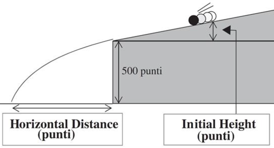
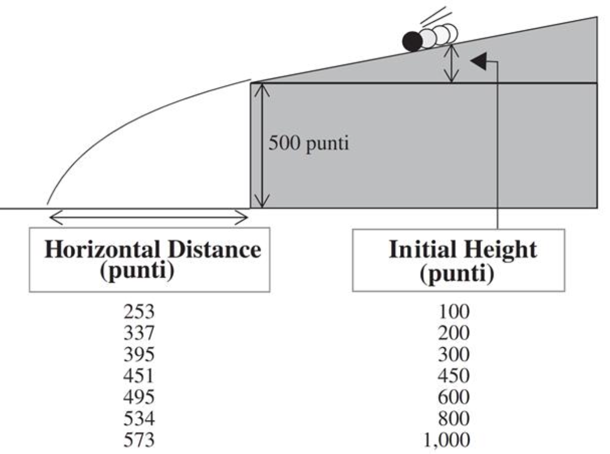
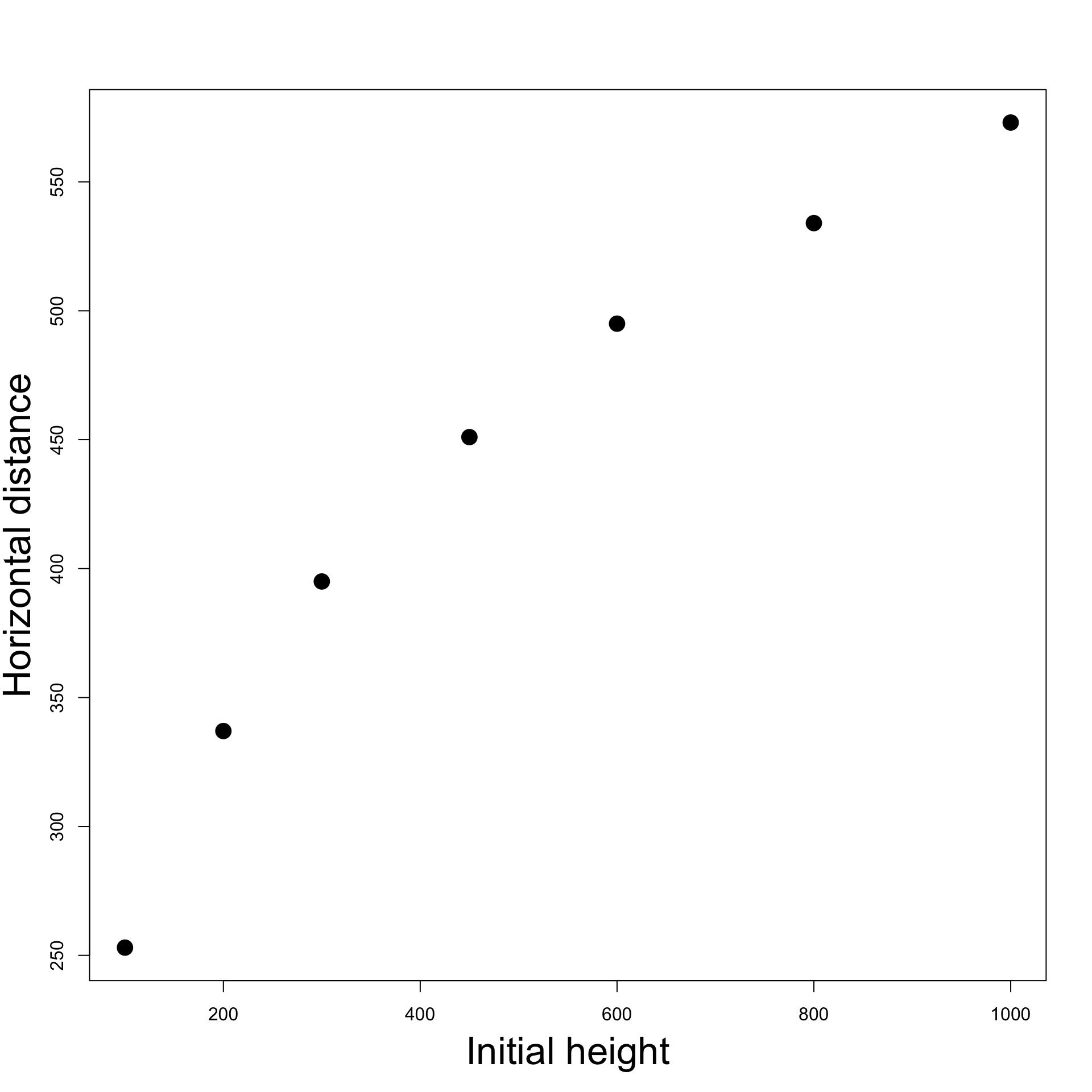
Example 2: Motion of falling bodies
Engraving (1546): people believed projectiles follow circular trajectories (source )
1609: Galileo proved mathematically that projectile trajectories are parabolic
His finding was based on empirical data
A ball (covered in ink) was released on an inclined plane from Initial Height
Ink mark on the floor represented the Horizontal Distance traveled
Unit of measure is punti \qquad\quad 1 \text{ punto} = 169/180 \, \text{mm}
We have access to Galileo’s original data [3 ]
Does a parabolic (quadratic) trajectory really explain the data?
Let’s fit a polynomial regression model and find out!
Plotting the data
Horizontal Distance 253
337
395
451
495
534
573
# Enter the data <- c (100 , 200 , 300 , 450 , 600 , 800 , 1000 )<- c (253 , 337 , 395 , 451 , 495 , 534 , 573 )# Scatter plot of data plot (height, distance, pch = 16 )
We clearly see a parabola. Therefore we expect a relation of the form
{\rm distance} = \beta_1 + \beta_2 \, {\rm height } + \beta_3 \, {\rm height }^2
Fit linear model
{\rm distance} = \beta_1 + \beta_2 \, {\rm height }
# Fit linear model <- lm (distance ~ height)summary (linear)
Multiple R-squared: 0.9264, Adjusted R-squared: 0.9116
The coefficient of correlation is R^2 = 0.9264
R^2 is quite high, showing that a linear model fits reasonably well
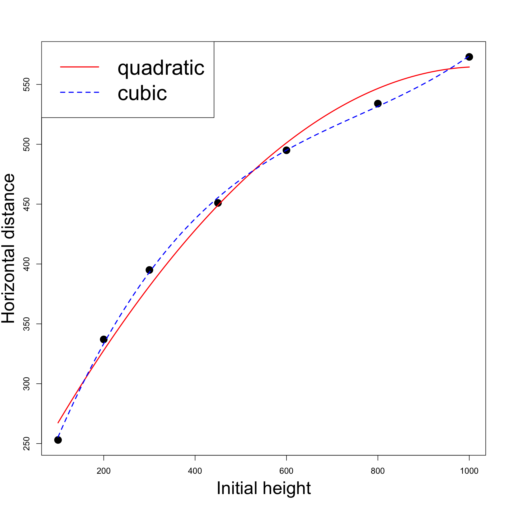
Is a quadratic model better?
{\rm distance} = \beta_1 + \beta_2 \, {\rm height } + \beta_3
\, {\rm height }^2
Note: To specify powers we need to type \,\, \texttt{I}
# Fit quadratic model <- lm (distance ~ height + I ( height^ 2 ))summary (quadratic)
Multiple R-squared: 0.9903, Adjusted R-squared: 0.9855
The coefficient of correlation is R^2 = 0.9903
This is higher than the previous score R^2 = 0.9264
The quadratic trajectory explains 99\% of variability in the data
Why not try a cubic model?
{\rm distance} = \beta_1 + \beta_2 \, {\rm height } + \beta_3
\, {\rm height }^2 + \beta_4 \, {\rm height }^3
# Fit cubic model <- lm (distance ~ height + I ( height^ 2 ) + I (height^ 3 ))summary (cubic)
Multiple R-squared: 0.9994, Adjusted R-squared: 0.9987
The coefficient of correlation is R^2 = 0.9994
This is higher than the score of quadratic model R^2 = 0.9903
What is going on?
Quadratic vs cubic
# Model selection anova (quadratic, cubic, test = "F" )
Analysis of Variance Table

Model 1: distance ~ height + I(height^2)
Model 2: distance ~ height + I(height^2) + I(height^3)
  Res.Df    RSS Df Sum of Sq     F  Pr(>F)
1      4 744.08
2      3  48.25  1    695.82 43.26 0.00715 **
Model selection: quadratic Vs cubic
\beta_4 = 0
Therefore the quadratic model does not describe the data well
The underlying relationship from Galileo’s data is cubic and not quadratic
Probably the inclined plane introduced drag
Code can be downloaded here galileo.R
Plot: Quadratic Vs Cubic
Click here for full code
# Enter the data <- c (100 , 200 , 300 , 450 , 600 , 800 , 1000 )<- c (253 , 337 , 395 , 451 , 495 , 534 , 573 )# Scatter plot of data plot (height, distance, xlab = "" , ylab = "" , pch = 16 , cex = 2 )# Add labels mtext ("Initial height" , side = 1 , line = 3 , cex = 2.1 )mtext ("Horizontal distance" , side = 2 , line = 2.5 , cex = 2.1 )# Fit quadratic model <- lm (distance ~ height + I ( height^ 2 ))# Fit cubic model <- lm (distance ~ height + I ( height^ 2 ) + I (height^ 3 ))# Plot quadratic Vs Cubic <- Vectorize (function (x, ps) {<- length (ps)sum (ps* x^ (1 : n-1 ))"x" )curve (polynomial (x, coef (quadratic)), add= TRUE , col = "red" , lwd = 2 )curve (polynomial (x, coef (cubic)), add= TRUE , col = "blue" , lty = 2 , lwd = 2 )legend ("topleft" , legend = c ("quadratic" , "cubic" ), col = c ("red" , "blue" ), lty = c (1 ,2 ), lwd = 2 , cex = 2.5 )
Why not try higher degree polynomials
{\rm distance} = \beta_1 + \beta_2 \, {\rm height } + \beta_3
\, {\rm height }^2 + \beta_4 \, {\rm height }^3
+ \beta_5 \, {\rm height }^4
# Fit quartic model <- lm (distance ~ height + I ( height^ 2 ) + I (height^ 3 ) + I (height^ 4 ))summary (quartic)
Multiple R-squared: 0.9998, Adjusted R-squared: 0.9995
We obtain a coefficient R^2 = 0.9998
This is even higher than cubic model coefficient R^2 = 0.9994
Is the quartic model actually better?
Model selection: cubic Vs quartic
# Model selection anova (cubic, quartic, test = "F" )
Analysis of Variance Table

Model 1: distance ~ height + I(height^2) + I(height^3)
Model 2: distance ~ height + I(height^2) + I(height^3) + I(height^4)
  Res.Df    RSS Df Sum of Sq      F Pr(>F)
1      3 48.254
2      2 12.732  1    35.522 5.5799  0.142
The F-test is not significant since p = 0.142 > 0.05
This means we cannot reject the null hypothesis that \beta_5 = 0
The cubic models does better than quartic, despite higher R^2
The underlying relationship from Galileo’s data is indeed cubic!
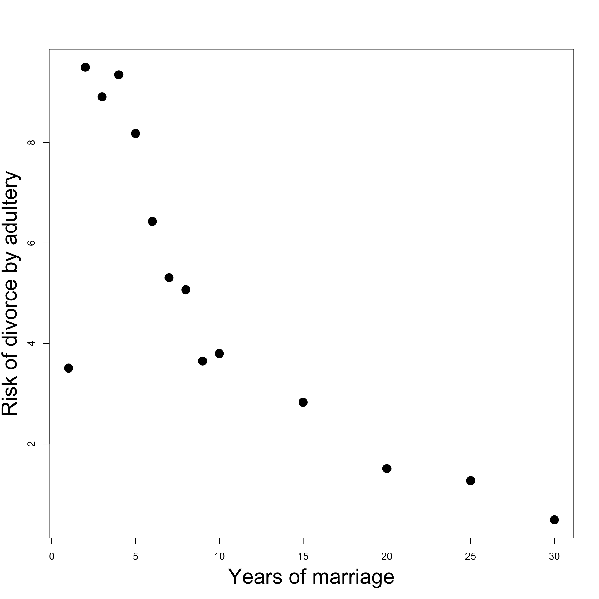
Example 3: Divorces
Data from Daily Mirror gives
Percentage of divorces caused by adultery VS years of marriage
Original analysis claimed
Divorce-risk peaks at year 2 then decreases thereafter
Is this conclusion misleading?
Does a quadratic model offers a better fit than a straight line model?
Divorces dataset
Percent of divorces caused by adultery by year of marriage
% divorces adultery 3.51
9.50
8.91
9.35
8.18
6.43
5.31
% divorces adultery 5.07
3.65
3.80
2.83
1.51
1.27
0.49
Plot: Years of Marriage Vs Divorce-risk
Looks like: Divorce-risk is
First low,
then peaks at year 2
then decreases
Change of trend suggests:
Higher order model might be good fit
Consider quadratic model
Click here for full code
# Divorces data <- c (1 , 2 , 3 , 4 , 5 , 6 ,7 , 8 , 9 , 10 , 15 , 20 , 25 , 30 )<- c (3.51 , 9.5 , 8.91 , 9.35 , 8.18 , 6.43 , 5.31 , 5.07 , 3.65 , 3.8 , 2.83 , 1.51 , 1.27 , 0.49 )# Scatter plot of data plot (year, percent, xlab = "" , ylab = "" , pch = 16 , cex = 2 )# Add labels mtext ("Years of marriage" , side = 1 , line = 3 , cex = 2.1 )mtext ("Risk of divorce by adultery" , side = 2 , line = 2.5 , cex = 2.1 )
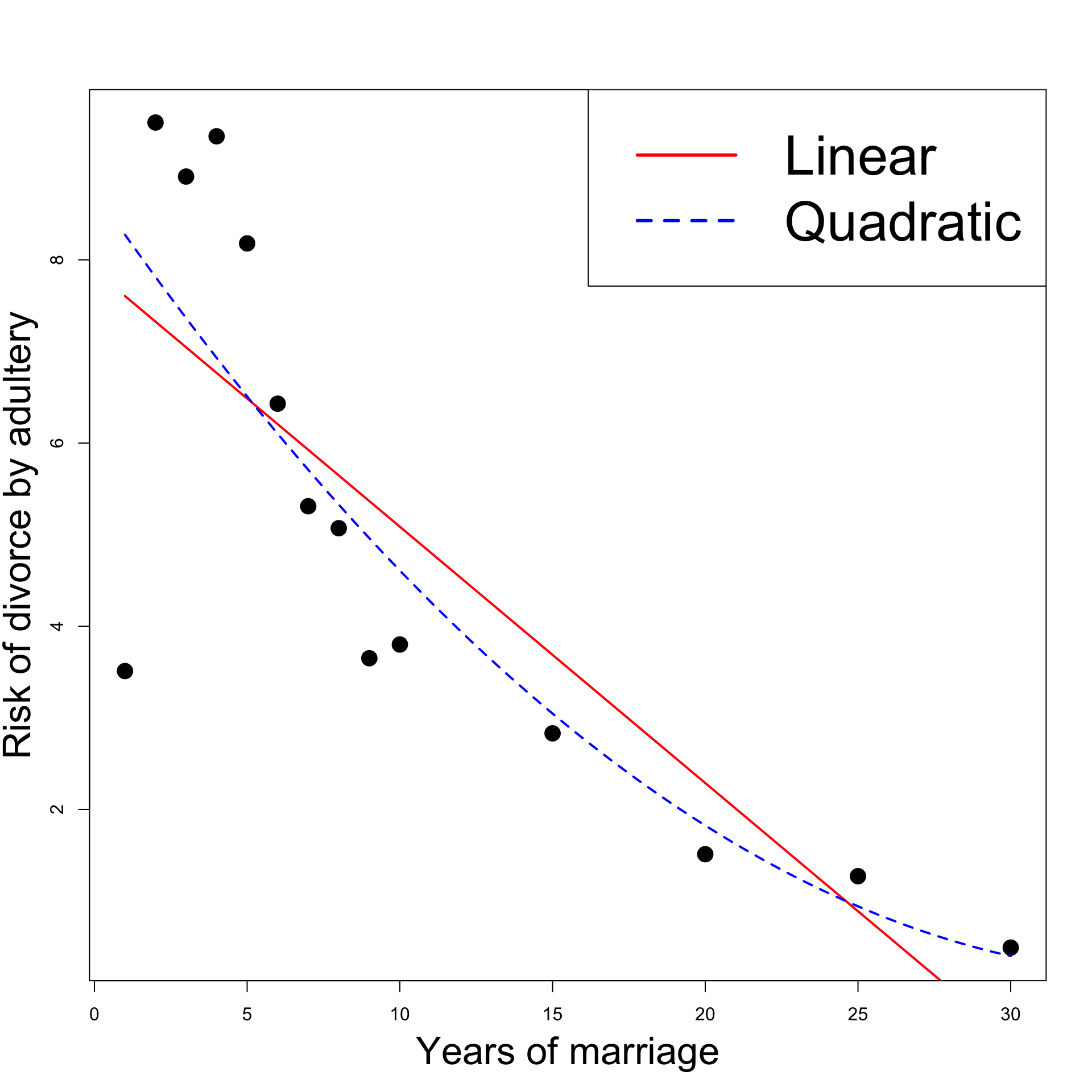
Fitting linear model
# Divorces data <- c (1 , 2 , 3 , 4 , 5 , 6 ,7 , 8 , 9 , 10 , 15 , 20 , 25 , 30 )<- c (3.51 , 9.5 , 8.91 , 9.35 , 8.18 , 6.43 , 5.31 , 5.07 , 3.65 , 3.8 , 2.83 , 1.51 , 1.27 , 0.49 )# Fit linear model <- lm (percent ~ year)summary (linear)
            Estimate Std. Error t value Pr(>|t|)
(Intercept)  7.88575    0.78667  10.024 3.49e-07 ***
year        -0.27993    0.05846  -4.788 0.000442 ***
t-test for \beta_2 is significant since p = 0.0004 < 0.05
Therefore \beta_2 \neq 0 and the estimate is \hat \beta_2 = -0.27993
The risk of divorce decreases with years of marriage (because \hat \beta_2 < 0 )
Fitting quadratic model
# Fit quadratic model <- lm (percent ~ year + I ( year^ 2 ))summary (quadratic)
             Estimate Std. Error t value Pr(>|t|)
(Intercept)  8.751048   1.258038   6.956  2.4e-05 ***
year        -0.482252   0.235701  -2.046   0.0654 .
I(year^2)    0.006794   0.007663   0.887   0.3943
t-test for \beta_3 is not significant since p = 0.3943 > 0.05
Cannot reject null hypothesis \beta_3 = 0 \quad \implies \quad Quadratic term not needed!
The original analysis in the Daily Mirror is probably mistaken
Model selection: Linear Vs Quadratic
# Model selection anova (linear, quadratic, test = "F" )
Model 1: percent ~ year
Model 2: percent ~ year + I(year^2)
  Res.Df    RSS Df Sum of Sq     F Pr(>F)
1     12 42.375
2     11 39.549  1     2.826 0.786 0.3943
F-test is not significant since p = 0.3943 > 0.05
We cannot reject the null hypothesis that \beta_3 = 0
Quadratic model is worse than linear model
Conclusions
Daily Mirror Claim: Divorce-risk peaks at year 2 then decreases thereafter
Claim suggests higher order model needed to explain change in trend
Analysis conducted:
Fit linear and quadratic regression models
t-test of significance discarded quadratic term
F-test for model selection discarded Quadratic model
Findings: Claims in Daily Mirror are misleading
Linear model seems to be better than quadratic
This suggests divorce-risk generally decreases over time
Peak in year 2 can be explained by unusually low divorce-risk in 1st year
Code is available here divorces.R
Click here for full code
# Divorces data <- c (1 , 2 , 3 , 4 , 5 , 6 ,7 , 8 , 9 , 10 , 15 , 20 , 25 , 30 )<- c (3.51 , 9.5 , 8.91 , 9.35 , 8.18 , 6.43 , 5.31 , 5.07 , 3.65 , 3.8 , 2.83 , 1.51 , 1.27 , 0.49 )# Fit linear model <- lm (percent ~ year)# Fit quadratic model <- lm (percent ~ year + I ( year^ 2 ))# Scatter plot of data plot (year, percent, xlab = "" , ylab = "" , pch = 16 , cex = 2 )# Add labels mtext ("Years of marriage" , side = 1 , line = 3 , cex = 2.1 )mtext ("Risk of divorce by adultery" , side = 2 , line = 2.5 , cex = 2.1 )# Plot Linear Vs Quadratic <- Vectorize (function (x, ps) {<- length (ps)sum (ps* x^ (1 : n-1 ))"x" )curve (polynomial (x, coef (linear)), add= TRUE , col = "red" , lwd = 2 )curve (polynomial (x, coef (quadratic)), add= TRUE , col = "blue" , lty = 2 , lwd = 2 )legend ("topright" , legend = c ("Linear" , "Quadratic" ), col = c ("red" , "blue" ), lty = c (1 ,2 ), cex = 3 , lwd = 3 )
Why not try higher order polynomials
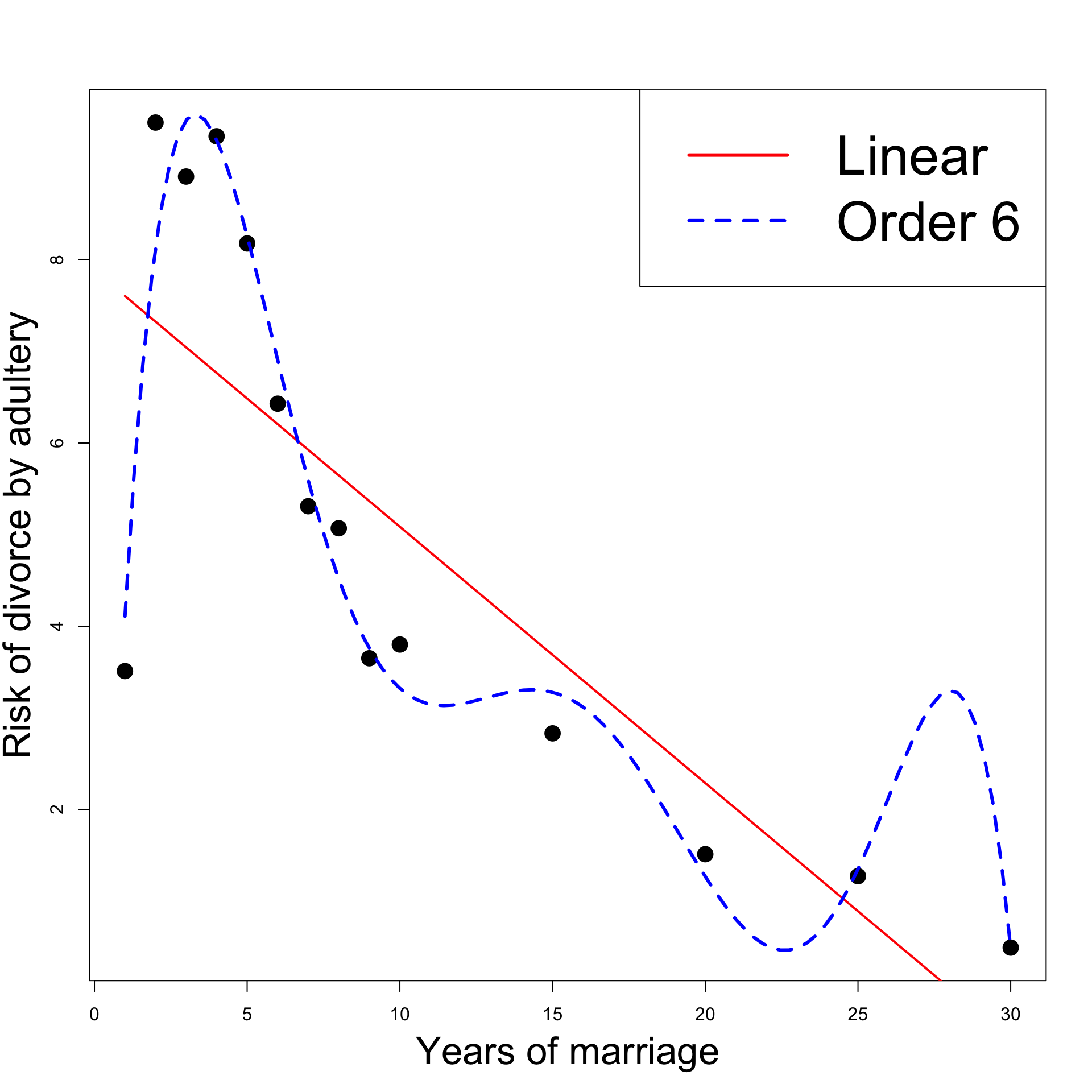
Let us compare Linear model with Order 6 Model
# Fit order 6 model <- lm (percent ~ year + I ( year^ 2 ) + I ( year^ 3 ) + + I ( year^ 4 ) + I ( year^ 5 ) + + I ( year^ 6 ))# Model selection anova (linear, order_6)
Model 1: percent ~ year
Model 2: percent ~ year + I(year^2) + I(year^3) + I(year^4) + I(year^5) +
    +I(year^6)
  Res.Df    RSS Df Sum of Sq      F   Pr(>F)
1     12 42.375
2      7  3.724  5    38.651 14.531 0.001404 **
Why not try higher order polynomials
\beta_3 = \beta_4 = \beta_5 = \beta_6 = 0
The Order 6 model is better than the Linear model
Peak divorce-rate in Year 2 is well explained by order 6 regression
What is going on? Let us plot the regression functions
There are more peaks:
Decreasing risk of divorce for 23 years
But it gets boring after 27 years!
Model overfits :
Data is very well explained
but predictions are not realistic
Linear model should be preferred
Click here for full code
# Divorces data <- c (1 , 2 , 3 , 4 , 5 , 6 ,7 , 8 , 9 , 10 , 15 , 20 , 25 , 30 )<- c (3.51 , 9.5 , 8.91 , 9.35 , 8.18 , 6.43 , 5.31 , 5.07 , 3.65 , 3.8 , 2.83 , 1.51 , 1.27 , 0.49 )# Fit linear model <- lm (percent ~ year)# Fit order 6 model <- lm (percent ~ year + I ( year^ 2 ) + I ( year^ 3 ) + I ( year^ 4 ) + I ( year^ 5 ) + I ( year^ 6 ))# Scatter plot of data plot (year, percent, xlab = "" , ylab = "" , pch = 16 , cex = 2 )# Add labels mtext ("Years of marriage" , side = 1 , line = 3 , cex = 2.1 )mtext ("Risk of divorce by adultery" , side = 2 , line = 2.5 , cex = 2.1 )# Plot Linear Vs Quadratic <- Vectorize (function (x, ps) {<- length (ps)sum (ps* x^ (1 : n-1 ))"x" )curve (polynomial (x, coef (linear)), add= TRUE , col = "red" , lwd = 2 )curve (polynomial (x, coef (order_6)), add= TRUE , col = "blue" , lty = 2 , lwd = 3 )legend ("topright" , legend = c ("Linear" , "Order 6" ), col = c ("red" , "blue" ), lty = c (1 ,2 ), cex = 3 , lwd = 3 )