Statistical Models

Lecture 1

Dr. Silvio Fanzon

S.Fanzon@hull.ac.uk

University of Hull

Dr. John Fry

J.M.Fry@hull.ac.uk

University of Hull

Lecture 1:
An introduction to Statistics

Outline of Lecture 1

1. Module info
2. Introduction
3. Probability revision
4. Moment generating functions

Part 1:
Module info

Contact details

• Lecturer: Dr. Silvio Fanzon
• Call me:
  • Silvio
  • Dr. Fanzon
• Email: S.Fanzon@hull.ac.uk
• Office: Room 104a, Larkin Building
• Office hours: Wednesday 12:00-13:00
• Meetings: in my office or send me an Email

Questions

• If you have any questions please feel free to email me

• We will address Homework and Coursework in class

• In addition, please do not hesitate to attend office hours

Lectures

Each week we have

• 2 Lectures of 2h each
• 1 Tutorial of 1h

Session	Date	Place
Lecture 1	Wed 10:00-12:00	Wilberforce LR 22
Lecture 2	Thu 15:00-17:00	Wilberforce LR 10
Tutorial	Thu 11:00-12:00	Wilberforce LR 7

Assessment

This course will be assessed as follows:

Type of Assessment	Percentage of final grade
Coursework Portfolio	70%
Homework	30%

Rules for Coursework

• Coursework available on Canvas from Week 3

• We will discuss coursework exercises in class

• Coursework must be submitted on Canvas

• Deadline: 14:00 on Thursday 2nd May

Rules for Homework

• 10 Homework papers, posted weekly on Canvas

• Each Homework paper is worth 14 points

• Final Homework grade computation:

  • Sum the top 7 scores (max score 98 points)
  • Bonus 2 points will be added to the final score

• Homework papers must be submitted on Canvas

• Deadlines: 14:00 on Mondays

Key submission dates

Assignment	Due date
Homework 1	5 Feb
Homework 2	12 Feb
Homework 3	19 Feb
Homework 4	26 Feb
Homework 5	4 Mar
Homework 6	11 Mar

Assignment	Due date
Homework 7	18 Mar
Easter Break	😎
Homework 8	8 Apr
Homework 9	15 Apr
Homework 10	22 Apr
Coursework	2 May

How to submit assignments

• Submit PDFs only on Canvas

• You have two options:

  • Write on tablet and submit PDF Output
  • Write on paper and Scan in Black and White using a Scanner or Scanner App (Tiny Scanner, Scanner Pro, …)

Important: I will not mark

• Assignments submitted outside of Canvas
• Assignments submitted After the Deadline

References

Main textbooks

Slides are self-contained and based on the book

• [1] Bingham, N. H. and Fry, J. M.
  Regression: Linear models in statistics.
  Springer, 2010

References

Main textbooks

.. and also on the book

• [2] Fry, J. M. and Burke, M.
  Quantitative methods in finance using R.
  Open University Press, 2022

References

Secondary References

• [3] Casella, G. and Berger R. L.
  Statistical inference.
  Second Edition, Brooks/Cole, 2002

• [4] DeGroot M. H. and Schervish M. J.
  Probability and Statistics.
  Fourth Edition, Addison-Wesley, 2012

Probability & Statistics manual

Easier Probability & Statistics manual

References

Secondary References

• [5] Dalgaard, P.
  Introductory statistics with R.
  Second Edition, Springer, 2008

• [6] Davies, T. M.
  The book of R.
  No Starch Press, 2016

Concise Statistics with R

Comprehensive R manual

Part 2:
Introduction

The nature of Statistics

Statistics is a mathematical subject

• Maths skills will give you a head start

• There are other occasions where common sense and detective skills can be more important

• Provides an early example of mathematics working in concert with the available computation

The nature of Statistics

We will use a combination of hand calculation and software

• Recognises that you are maths students
• Software (R) is really useful, particularly for dissertations
• Please bring your laptop into class
• Download R onto your laptop

Overview of the module

Module has 11 Lectures, divided into two parts:

• Part I - Mathematical statistics

• Part II - Applied statistics

Overview of the module

Part I - Mathematical statistics

1. Introduction to statistics
2. Normal distribution family and one-sample hypothesis tests
3. Two-sample hypothesis tests
4. The chi-squared test
5. Non-parametric statistics
6. The maths of regression

Overview of the module

Part II - Applied statistics

7. An introduction to practical regression
8. The extra sum of squares principle and regression modelling assumptions
9. Violations of regression assumptions – Autocorrelation
10. Violation of regression assumptions – Multicollinearity
11. Dummy variable regression models

Simple but useful questions

Generic data:

• What is a typical observation
  • What is the mean?
• How spread out is the data?
  • What is the variance?

Regression:

• What happens to Y as X increases?
  • increases?
  • decreases?
  • nothing?

Statistics answers these questions systematically

• important for large datasets
• The same mathematical machinery (normal family of distributions) can be applied to both questions

Analysing a general dataset

Two basic questions:

1. Location or mean
2. Spread or variance

Statistics enables to answer systematically:

1. One sample and two-sample t-test
2. Chi-squared test and F-test

Recall the following sketch

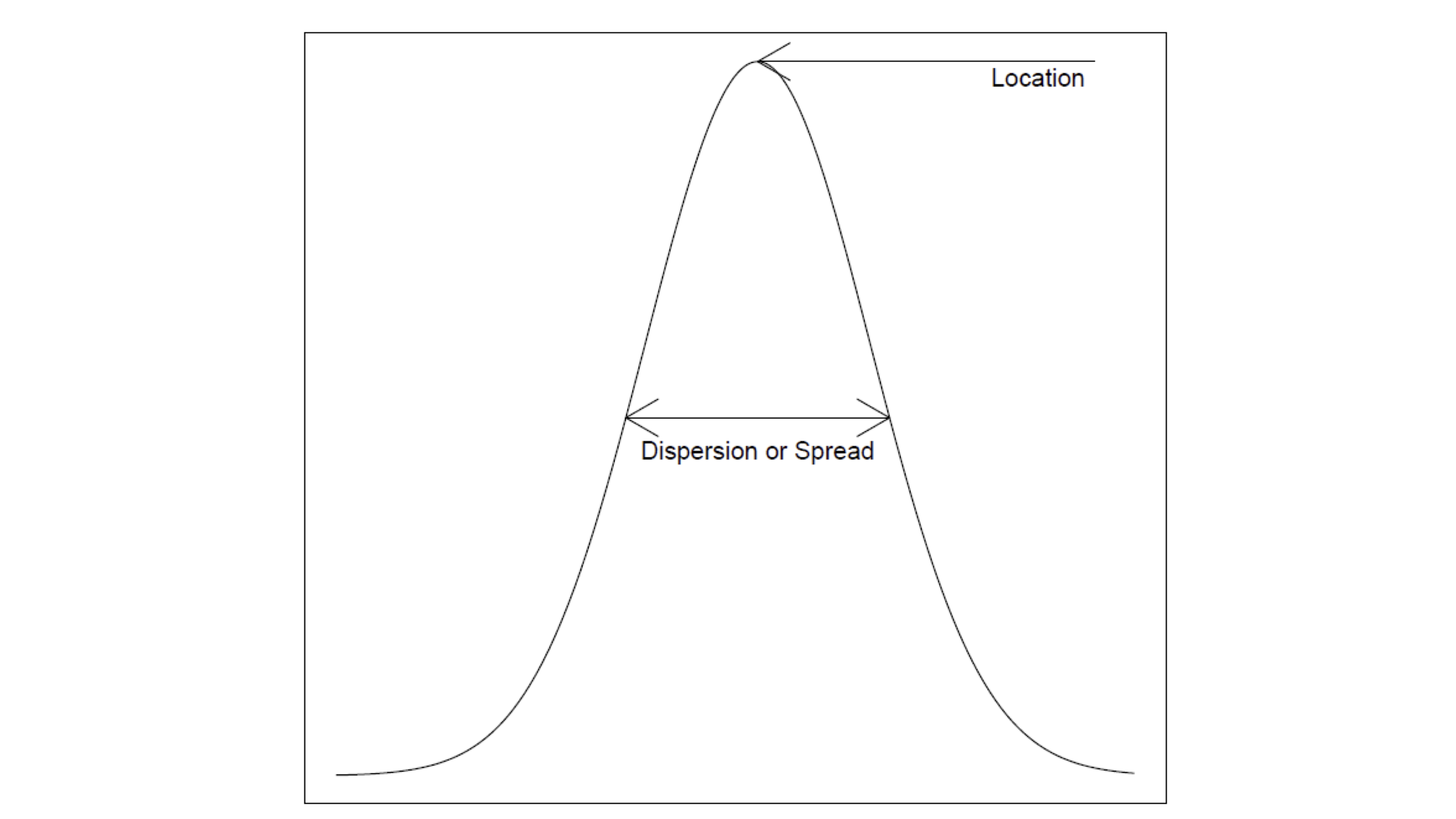
Curve represents data distribution

Motivating regression

Basic question in regression:

• What happens to Y as X increases?

  • increases?
  • decreases?
  • nothing?

In this way regression can be seen as a more advanced version of high-school maths

Positive gradient

As X increases Y increases

Negative gradient

As X increases Y decreases

Zero gradient

Changes in X do not affect Y

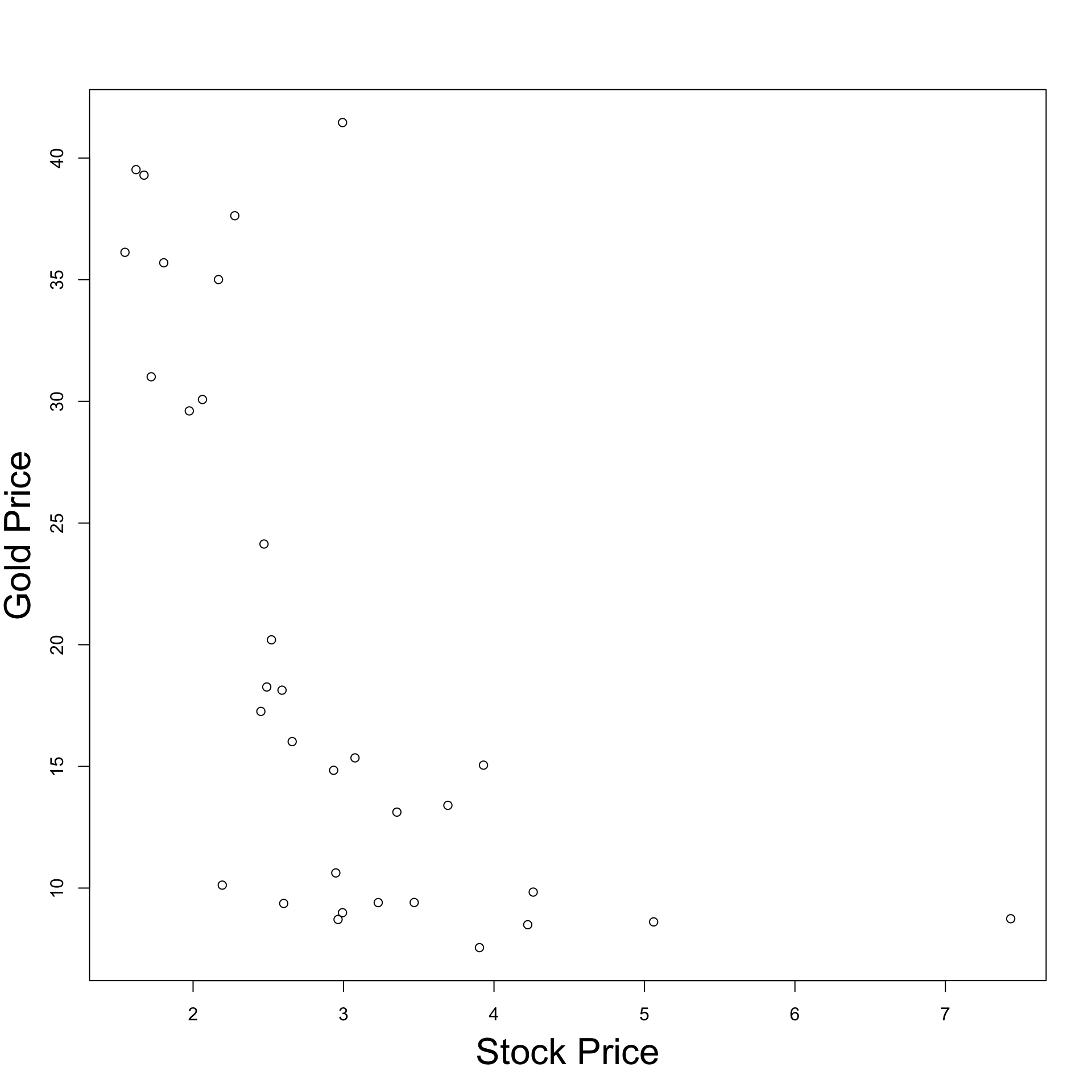
Real data example

• Real data is more imperfect
• But the same basic idea applies
• Example:
  • X = Stock price
  • Y = Gold price

Real data example

How does real data look like?

Dataset with 33 entries for Stock and Gold price pairs

Stock Price Gold Price 1 3.230426 9.402434 2 2.992937 8.987918 3 2.194025 10.120387 4 2.602475 9.367327 5 2.963497 8.708742 6 4.224242 8.494215 7 7.433981 8.739684 8 5.060836 8.609681 9 3.903316 7.552746 10 4.260542 9.834538 11 3.469490 9.406448

Stock Price Gold Price 12 2.948513 10.62240 13 3.354562 13.12062 14 3.930106 15.05097 15 3.693491 13.39932 16 3.076129 15.34968 17 2.934277 14.83910 18 2.658664 16.01850 19 2.450606 17.25952 20 2.489758 18.26270 21 2.591093 18.13104 22 2.520800 20.20052

Stock Price Gold Price 23 2.471447 24.13767 24 2.062430 30.07695 25 1.805153 35.69485 26 1.673950 39.29658 27 1.620848 39.52317 28 1.547374 36.12564 29 1.721679 31.01106 30 1.974891 29.60810 31 2.168978 35.00593 32 2.277214 37.62929 33 2.993353 41.45828

Real data example

Visualizing the data

• Plot Stock Price against Gold Price

• Observation:

  • As Stock price decreases, Gold price increases

• Why? This might be because:

  • Stock price decreases
  • People invest in secure assets (Gold)
  • Gold demand increases
  • Gold price increases

Don’t panic

• Regression problems can look a lot harder than they really are
  • Basic question remains the same: what happens to Y as X increases?
• Beware of jargon. Various authors distinguish between
  • Two variable regression model
  • Multiple regression model
  • Analysis of Variance
  • Analysis of Covariance
• Despite these apparent differences:
  • Mathematical methodology stays (essentially) the same
  • regression-fitting commands in R stay (essentially) the same

Part 3:
Probability revision

Probability revision

• We start with reviewing some fundamental Probability notions
• You saw these in the Y1 module Introduction to Probability & Statistics
• We will adopt a slightly more mature mathematical approach
• Remember: The mathematical description might look (a bit) different, but the concepts are the same

Topics reviewed:

• Sample space
• Events
• Probability measure
• Conditional probability
• Events independence

• Random Variable
• Distribution
• cdf
• pmf
• pdf

Sample space

Definition: Sample space

A set \Omega of all possible outcomes of some experiment

Examples:

• Coin toss: results in Heads = H and Tails = T \Omega = \{ H, T \}

• Student grade for Statistical Models: a number between 0 and 100 \Omega = \{ x \in \mathbb{R} \, \colon \, 0 \leq x \leq 100 \} = [0,100]

Events

Definition: Event

A subset E of the sample space \Omega (including \emptyset and \Omega itself)

Operations with events:

• Union of two events A and B A \cup B := \{ x \in \Omega \colon x \in A \, \text{ or } \, x \in B \}

• Intersection of two events A and B A \cap B := \{ x \in \Omega \colon x \in A \, \text{ and } \, x \in B \}

Events

More Operations with events:

• Complement of an event A A^c := \{ x \in \Omega \colon x \notin A \}

• Infinite Union of a family of events A_i with i \in I

\bigcup_{i \in I} A_i := \{ x \in \Omega \colon x \in A_i \, \text{ for some } \, i \in I \}

• Infinite Intersection of a family of events A_i with i \in I

\bigcap_{i \in I} A_i := \{ x \in \Omega \colon x \in A_i \, \text{ for all } \, i \in I \}

Events

Example: Consider sample space and events \Omega := (0,1] \,, \quad A_i = \left[\frac{1}{i} , 1 \right] \,, \quad i \in \mathbb{N} Then \bigcup_{i \in I} A_i = (0,1] \,, \quad \bigcap_{i \in I} A_i = \{ 1 \}

Events

Definition: Disjoint

Two events A and B are disjoint if A \cap B = \emptyset Events A_1, A_2, \ldots are pairwise disjoint if A_i \cap A_j = \emptyset \,, \quad \forall \, i \neq j

Events

Definition: Partition

The collection of events A_1, A_2, \ldots is a partition of \Omega if

1. A_1, A_2, \ldots are pairwise disjoint
2. \Omega = \cup_{i=1}^\infty A_i

What’s a Probability?

• To each event E \subset \Omega we would like to associate a number P(E) \in [0,1]

• The number P(E) is called the probability of E

• The number P(E) models the frequency of occurrence of E:

  • P(E) small means E has low chance of occurring
  • P(E) large means E has high chance of occurring

• Technical issue:

  • One cannot associate a number P(E) for all events in \Omega
  • Probability function P only defined for a smaller family of events
  • Such family of events is called \sigma-algebra

\sigma-algebras

Definition: sigma-algebra

Let \mathcal{B} be a collection of events. We say that \mathcal{B} is a \sigma-algebra if

1. \emptyset \in \mathcal{B}
2. If A \in \mathcal{B} then A^c \in \mathcal{B}
3. If A_1,A_2 , \ldots \in \mathcal{B} then \cup_{i=1}^\infty A_i \in \mathcal{B}

Remarks:

• Since \emptyset \in \mathcal{B} and \emptyset^c = \Omega, we deduce that \Omega \in \mathcal{B}

• Thanks to DeMorgan’s Law we have that A_1,A_2 , \ldots \in \mathcal{B} \quad \implies \quad \cap_{i=1}^\infty A_i \in \mathcal{B}

\sigma-algebras

Examples

Suppose \Omega is any set:

• Then \mathcal{B} = \{ \emptyset, \Omega \} is a \sigma-algebra

• The power set of \Omega \mathcal{B} = \operatorname{Power} (\Omega) := \{ A \colon A \subset \Omega \} is a \sigma-algebra

\sigma-algebras

Examples

• If \Omega has n elements then \mathcal{B} = \operatorname{Power} (\Omega) contains 2^n sets

• If \Omega = \{ 1,2,3\} then \begin{align*} \mathcal{B} = \operatorname{Power} (\Omega) = \big\{ & \{1\} , \, \{2\}, \, \{3\} \\ & \{1,2\} , \, \{2,3\}, \, \{1,3\} \\ & \emptyset , \{1,2,3\} \big\} \end{align*}

• If \Omega is uncountable then the power set of \Omega is not easy to describe

Lebesgue \sigma-algebra

Question

\mathbb{R} is uncountable. Which \sigma-algebra do we consider?

Definition: Lebesgue sigma-algebra

The Lebesgue \sigma-algebra on \mathbb{R} is the smallest \sigma-algebra \mathcal{L} containing all sets of the form (a,b) \,, \quad (a,b] \,, \quad [a,b) \,, \quad [a,b] for all a,b \in \mathbb{R}

Lebesgue \sigma-algebra

Important

Therefore the events of \mathbb{R} are

• Intervals
• Unions and intersection of intervals
• Countable Unions and intersection of intervals

Warning

• I only told you that the Lebsesgue \sigma-algebra \mathcal{L} exists
• Explicitly showing that \mathcal{L} exists is not easy, see [7]

Probability measure

Suppose given:

• \Omega sample space
• \mathcal{B} a \sigma-algebra on \Omega

Definition: Probability measure

A probability measure on \Omega is a map P \colon \mathcal{B} \to [0,1] such that the Axioms of Probability hold

1. P(\Omega) = 1
2. If A_1, A_2,\ldots are pairwise disjoint then P\left( \bigcup_{i=1}^\infty A_i \right) = \sum_{i=1}^\infty P(A_i)

Properties of Probability

Let A, B \in \mathcal{B}. As a consequence of the Axioms of Probability:

1. P(\emptyset) = 0
2. If A and B are disjoint then P(A \cup B) = P(A) + P(B)
3. P(A^c) = 1 - P(A)
4. P(A) = P(A \cap B) + P(A \cap B^c)
5. P(A\cup B) = P(A) + P(B) - P(A \cap B)
6. If A \subset B then P(A) \leq P(B)

Properties of Probability

7. Suppose A is an event and B_1,B_2, \ldots a partition of \Omega. Then P(A) = \sum_{i=1}^\infty P(A \cap B_i)
8. Suppose A_1,A_2, \ldots are events. Then P\left( \bigcup_{i=1}^\infty A_i \right) \leq \sum_{i=1}^\infty P(A_i)

Example: Fair Coin Toss

• The sample space for coin toss is \Omega = \{ H, T \}

• We take as \sigma-algebra the power set of \Omega \mathcal{B} = \{ \emptyset , \, \{H\} , \, \{T\} , \, \{H,T\} \}

• We suppose that the coin is fair

  • This means P \colon \mathcal{B} \to [0,1] satisfies P(\{H\}) = P(\{T\})
  • Assuming the above we get 1 = P(\Omega) = P(\{H\} \cup \{T\}) = P(\{H\}) + P(\{T\}) = 2 P(\{H\})
  • Therefore P(\{H\}) = P(\{T\}) = \frac12

Conditional Probability

Definition: Conditional Probability

Let A,B be events in \Omega with P(B)>0 The conditional probability of A given B is P(A|B) := \frac{P(A \cap B)}{P(B)}

Conditional Probability

Intuition

The conditional probability P(A|B) = \frac{P( A \cap B)}{P(B)} represents the probability of A, knowing that B has happened:

• If B has happened, then B is the new sample space
• Therefore A \cap B^c cannot happen, and we are only interested in A \cap B
• Hence it makes sense to define P(A|B) \propto P(A \cap B)
• We divide P(A\cap B) by P(B) so that P(A|B) \in [0,1] is still a probability
• The function A \mapsto P(A|B) is a probability measure on \Omega

Bayes’ Rule

• For two events A and B is holds

P(A | B ) = P(B|A) \frac{P(A)}{P(B)}

• Given a partition A_1, A_2, \ldots of the sample space we have

P(A_i | B ) = \frac{ P(B|A_i) P(A_i)}{\sum_{j=1}^\infty P(B | A_j) P(A_j)}

Independence

Definition

Two events A and B are independent if P(A \cap B) = P(A)P(B) A collection of events A_1 , \ldots ,A_n are mutually independent if for any subcollection A_{i_1}, \ldots, A_{i_k} it holds P \left( \bigcap_{j=1}^k A_j \right) = \prod_{j=1}^k P(A_{i_j})

Random Variables

Motivation

• Consider the experiment of flipping a coin 50 times
• The sample space consists of 2^{50} elements
• Elements are vectors of 50 entries recording the outcome H or T of each flip
• This is a very large sample space!

Suppose we are only interested in X = \text{ number of } \, H \, \text{ in } \, 50 \, \text{flips}

• Then the new sample space is the set of integers \{ 0,1,2,\ldots,50\}
• This is much smaller!
• X is called a Random Variable

Random Variables

Assume given

• \Omega sample space
• \mathcal{B} a \sigma-algebra of events on \Omega
• P \colon \mathcal{B} \to [0,1] a probability measure

Definition: Random variable

A function X \colon \Omega \to \mathbb{R}

We will abbreviate Random Variable with rv

Random Variables

Technical remark

Definition: Random variable

A measurable function X \colon \Omega \to \mathbb{R}

Technicality: X is a measurable function if \{ X \in I \} := \{ \omega \in \Omega \colon X(\omega) \in I \} \in \mathcal{B} \,, \quad \forall \, I \in \mathcal{L} where

• \mathcal{L} is the Lebsgue \sigma-algebra on \mathbb{R}
• \mathcal{B} is the given \sigma-algebra on \Omega

Random Variables

Notation

• In particular I \in \mathcal{L} can be of the form (a,b) \,, \quad (a,b] \,, \quad [a,b) \,, \quad [a,b] \,, \quad \forall \, a, b \in \mathbb{R}

• In this case the set \{X \in I\} \in \mathcal{B} is denoted by, respectively: \{ a < X < b \} \,, \quad \{ a < X \leq b \} \,, \quad \{ a \leq X < b \} \,, \quad \{ a \leq X \leq b \}

• If a=b=x then I=[x,x]=\{x\}. Then we denote \{X \in I\} = \{X = x\}

Distribution

Why do we require measurability?

Answer: Because it allows to define a new probability measure on \mathbb{R}

Definition: Distribution

The distribution of a random variable X \colon \Omega \to \mathbb{R} is the probability measure on \mathbb{R} P_X \colon \mathcal{L} \to [0,1] \,, \quad P_X (I) := P \left( \{X \in I\} \right) \,, \,\, \forall \, I \in \mathcal{L}

Note:

• One can show that P_X satisfies the Probability Axioms
• Thus P_X is a probability measure on \mathbb{R}
• In the future we will denote P \left( X \in I \right) := P \left( \{X \in I\} \right)

Distribution

Why is the distribution useful?

Answer: Because it allows to define a random variable X

• by specifying the distribution values P \left( X \in I \right)
• rather than defining an explicit function X \colon \Omega \to \mathbb{R}

Important: More often than not

• We care about the distribution of X
• We do not care about how X is defined

Example - Three coin tosses

• Sample space \Omega given by the below values of \omega

\omega

HHH

HHT

HTH

THH

TTH

THT

HTT

TTT

• The probability of each outcome is the same P(\omega) = \frac{1}{2} \times \frac{1}{2} \times \frac{1}{2} = \frac{1}{8} \,, \quad \forall \, \omega \in \Omega

• Define the random variable X \colon \Omega \to \mathbb{R} by X(\omega) := \text{ Number of H in } \omega

\omega	HHH	HHT	HTH	THH	TTH	THT	HTT	TTT
X(\omega)	3	2	2	2	1	1	1	0

Example - Three coin tosses

• Recall the definition of X

\omega	HHH	HHT	HTH	THH	TTH	THT	HTT	TTT
X(\omega)	3	2	2	2	1	1	1	0

• The range of X is \{0,1,2,3\}

• Hence the only interesting values of P_X are P(X=0) \,, \quad P(X=1) \,, \quad P(X=2) \,, \quad P(X=3)

Example - Three coin tosses

• Recall the definition of X

\omega	HHH	HHT	HTH	THH	TTH	THT	HTT	TTT
X(\omega)	3	2	2	2	1	1	1	0

• We compute \begin{align*} P(X=0) & = P(TTT) = \frac{1}{8} \\ P(X=1) & = P(TTH) + P(THT) + P(HTT) = \frac{3}{8} \\ P(X=2) & = P(HHT) + P(HTH) + P(THH) = \frac{3}{8} \\ P(X=3) & = P(HHH) = \frac{1}{8} \end{align*}

Example - Three coin tosses

• Recall the definition of X

\omega	HHH	HHT	HTH	THH	TTH	THT	HTT	TTT
X(\omega)	3	2	2	2	1	1	1	0

• The distribution of X is summarized in the table below

x	0	1	2	3
P(X=x)	\frac{1}{8}	\frac{3}{8}	\frac{3}{8}	\frac{1}{8}

Cumulative Distribution Function

Recall: The distribution of a rv X \colon \Omega \to \mathbb{R} is the probability measure on \mathbb{R} P_X \colon \mathcal{L} \to [0,1] \,, \quad P_X (I) := P \left( X \in I \right) \,, \,\, \forall \, I \in \mathcal{L}

Definition: cdf

The cumulative distribution function or cdf of a rv X \colon \Omega \to \mathbb{R} is F_X \colon \mathbb{R} \to \mathbb{R} \,, \quad F_X(x) := P_X (X \leq x)

Cumulative Distribution Function

Intuition

• F_X is the primitive of P_X:
  • Recall from Analysis: The primitive of a continuous function g \colon \mathbb{R}\to \mathbb{R} is G(x):=\int_{-\infty}^x g(y) \,dy
  • Note that P_X is not a function but a distribution
  • However the definition of cdf as a primitive still makes sense
• P_X will be the derivative of F_X - In a suitable generalized sense
  • Recall from Analysis: Fundamental Theorem of Calculus says G'(x)=g(x)
  • Since F_X is the primitive of P_X, it will still hold F_X'=P_X in the sense of distributions

Distribution Function

Example

• Consider again 3 coin tosses and the rv X(\omega) := \text{ Number of H in } \omega

• We computed that the distribution P_X of X is

x	0	1	2	3
P(X=x)	\frac{1}{8}	\frac{3}{8}	\frac{3}{8}	\frac{1}{8}

• One can compute F_X(x) = \begin{cases} 0 & \text{if } x < 0 \\ \frac{1}{8} & \text{if } 0 \leq x < 1 \\ \frac{1}{2} & \text{if } 1 \leq x < 2 \\ \frac{7}{8} & \text{if } 2 \leq x < 3 \\ 1 & \text{if } 3 \leq x \end{cases}

• For example \begin{align*} F_X(2.1) & = P(X \leq 2.1) \\ & = P(X=0,1 \text{ or } 2) \\ & = P(X=0) + P(X=1) + P(X=2) \\ & = \frac{1}{8} + \frac{3}{8} + \frac{3}{8} = \frac{7}{8} \end{align*}

Cumulative Distribution Function

Example

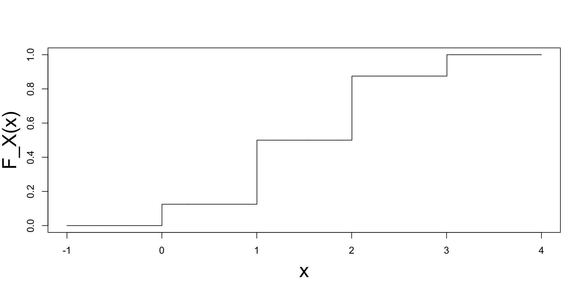
• Plot of F_X: it is a step function
• F_X'=0 except at x=0,1,2,3
• F_X jumps at x=0,1,2,3

• Size of jump at x is P(X=x)
• F_X'=P_X in the sense of distributions
  (Advanced analysis concept - not covered)

Discrete Random Variables

In the previous example:

• The cdf F_X had jumps
• Hence F_X was discountinuous
• We take this as definition of discrete rv

Definition

X \colon \Omega \to \mathbb{R} is discrete if F_X has jumps

Probability Mass Function

• In this slide X is a discrete rv
• Therefore F_X has jumps

Definition

The Probability Mass Function or pmf of a discrete rv X is f_X \colon \mathbb{R} \to \mathbb{R} \,, \quad f_X(x) := P(X = x)

Probability Mass Function

Properties

Proposition

The pmf f_X(x) = P(X=x) can be used to

• compute probabilities P(a \leq X \leq b) = \sum_{k = a}^b f_X (k) \,, \quad \forall \, a,b \in \mathbb{Z} \,, \,\, a \leq b
• compute the cdf F_X(x) = P(X \leq x) = \sum_{k=-\infty}^x f_X(k)

Example 1 - Discrete RV

• Consider again 3 coin tosses and the RV X(\omega) := \text{ Number of H in } \omega

• The pmf of X is f_X(x):=P(X=x), which we have already computed

x	0	1	2	3
f_X(x)= P(X=x)	\frac{1}{8}	\frac{3}{8}	\frac{3}{8}	\frac{1}{8}

Example 2 - Geometric Distribution

• Suppose p \in (0,1) is a given probability of success
• Hence 1-p is probability of failure
• Consider the random variable X = \text{ Number of attempts to obtain first success}
• Since each trial is independent, the pmf of X is f_X (x) = P(X=x) = (1-p)^{x-1} p \,, \quad \forall \, x \in \mathbb{N}
• This is called geometric distribution

Example 2 - Geometric Distribution

• We want to compute the cdf of X: For x \in \mathbb{N} with x > 0 \begin{align*} F_X(x) & = P(X \leq x) = \sum_{k=1}^x P(X=k) = \sum_{k=1}^x f_X(k) \\ & = \sum_{k=1}^x (1-p)^{k-1} p = \frac{1-(1-p)^x}{1-(1-p)} p = 1 - (1-p)^x \end{align*} where we used the formula for the sum of geometric series: \sum_{k=1}^x t^{k-1} = \frac{1-t^x}{1-t} \,, \quad t \neq 1

Example 2 - Geometric Distribution

• F_X is flat between two consecutive natural numbers: \begin{align*} F_X(x+k) & = P(X \leq x+k) \\ & = P(X \leq x) \\ & = F_X(x) \end{align*} for all x \in \mathbb{N}, k \in [0,1)

• Therefore F_X has jumps and X is discrete

Continuous Random Variables

Recall: X is discrete if F_X has jumps

Definition: Continuous Random Variable

X \colon \Omega \to \mathbb{R} is continuous if F_X is continuous

Probability Mass Function?

• Suppose X is a continuous rv
• Therefore F_X is continuous

Question

Can we define the Probability Mass Function for X?

Answer:

• Yes we can, but it would be useless - pmf carries no information
• This is because f_X(x) = P(X=x) = 0 \,, \quad \forall \, x \in \mathbb{R}

Probability Mass Function?

• Indeed, for all \varepsilon>0 we have \{ X = x \} \subset \{ x - \varepsilon < X \leq x \}
• Therefore by the properties of probabilities we have \begin{align*} P (X = x ) & \leq P( x - \varepsilon < X \leq x ) \\ & = P(X \leq x) - P(X \leq x - \varepsilon) \\ & = F_X(x) - F_X(x-\varepsilon) \end{align*} where we also used the definition of F_X
• Since F_X is continuous we get 0 \leq P(X = x) \leq \lim_{\varepsilon \to 0} F_X(x) - F_X(x-\varepsilon) = 0
• Then f_X(x) = P(X=x) = 0 for all x \in \mathbb{R}

Probability Density Function

• pmf carries no information for continuous RV
• We instead define the pdf

Definition

The Probability Density Function or pdf of a continuous rv X is a function f_X \colon \mathbb{R} \to \mathbb{R} s.t. F_X(x) = \int_{-\infty}^x f_X(t) \, dt \,, \quad \forall \, x \in \mathbb{R}

Technical issue:

• If X is continuous then pdf does not exist in general
• Counterexamples are rare, therefore we will assume existence of pdf

Probability Density Function

Properties

Proposition

Suppose X is continuous rv. They hold

• The cdf F_X is continuous and differentiable (a.e.) with F_X' = f_X

• Probability can be computed via P(a \leq X \leq b) = \int_{a}^b f_X (t) \, dt \,, \quad \forall \, a,b \in \mathbb{R} \,, \,\, a \leq b

Example - Logistic Distribution

• The random variable X has logistic distribution if its pdf is f_X(x) = \frac{e^{-x}}{(1+e^{-x})^2}

Example - Logistic Distribution

• The random variable X has logistic distribution if its pdf is f_X(x) = \frac{e^{-x}}{(1+e^{-x})^2}

• The cdf can be computed to be F_X(x) = \int_{-\infty}^x f_X(t) \, dt = \frac{1}{1+e^{-x}}

• The RHS is known as logistic function

Example - Logistic Distribution

Application: Logistic function models expected score in chess (see Wikipedia)

• R_A is ELO rating of player A, R_B is ELO rating of player B
• E_A is expected score of player A: E_A := P(A \text{ wins}) + \frac12 P(A \text{ draws})
• E_A modelled by logistic function E_A := \frac{1}{1+ 10^{(R_B-R_A)/400} }
• Example: Beginner is rated 1000, International Master is rated 2400 R_{\rm Begin} = 1000, \quad R_{\rm IM}=2400 , \quad E_{\rm Begin} = \frac{1}{1 + 10^{1400/400}} = 0.00031612779

Characterization of pmf and pdf

Theorem

Let f \colon \mathbb{R} \to \mathbb{R}. Then f is pmf or pdf of a RV X iff

1. f(x) \geq 0 for all x \in \mathbb{R}
2. \sum_{x=-\infty}^\infty f(x) = 1 \,\,\, (pmf) \quad or \quad \int_{-\infty}^\infty f(x) \, dx = 1\,\,\, (pdf)

In the above setting:

• The RV X has distribution P(X = x) = f(x) \,\,\, \text{ (pmf) } \quad \text{ or } \quad P(a \leq X \leq b) = \int_a^b f(t) \, dt \,\,\, \text{ (pdf)}

• The symbol X \sim f denotes that X has distribution f

Summary - Random Variables

• Suppose X \colon \Omega \to \mathbb{R} is RV

• Cumulative Density Function (cdf): F_X(x) := P(X \leq x)

Discrete RV	Continuous RV
F_X has jumps	F_X is continuous
Probability Mass Function (pmf)	Probability Density Function (pdf)
f_X(x) := P(X=x)	f_X(x) := F_X'(x)
f_X \geq 0	f_X \geq 0
\sum_{x=-\infty}^\infty f_X(x) = 1	\int_{-\infty}^\infty f_X(x) \, dx = 1
F_X (x) = \sum_{k=-\infty}^x f_X(k)	F_X (x) = \int_{-\infty}^x f_X(t) \, dt
P(a \leq X \leq b) = \sum_{k = a}^{b} f_X(k)	P(a \leq X \leq b) = \int_a^b f_X(t) \, dt

Part 4:
Moment generating functions

Functions of Random Variables

• X \colon \Omega \to \mathbb{R} random variable and g \colon \mathbb{R} \to \mathbb{R} function
• Then Y:=g(X) \colon \Omega \to \mathbb{R} is random variable
• For A \subset \mathbb{R} we define the pre-image g^{-1}(A) := \{ x \in \mathbb{R} \colon g(x) \in A \}
• For A=\{y\} single element set we denote g^{-1}(\{y\}) = g^{-1}(y) = \{ x \in \mathbb{R} \colon g(x) = y \}
• The distribution of Y is P(Y \in A) = P(g(X) \in A ) = P(X \in g^{-1}(A))

Functions of Random Variables

Question: What is the relationship between f_X and f_Y?

• X discrete: Then Y is discrete and f_Y (y) = P(Y = y) = \sum_{x \in g^{-1}(y)} P(X=x) = \sum_{x \in g^{-1}(y)} f_X(x)

• X and Y continuous: Then \begin{align*} F_Y(y) & = P(Y \leq y) = P(g(X) \leq y) \\ & = P(\{ x \in \mathbb{R} \colon g(x) \leq y \} ) = \int_{\{ x \in \mathbb{R} \colon g(x) \leq y \}} f_X(t) \, dt \end{align*}

Functions of Random Variables

Issue: The below set may be tricky to compute \{ x \in \mathbb{R} \colon g(x) \leq y \}

However it can be easily computed if g is strictly monotone:

• g strictly increasing: Meaning that x_1 < x_2 \quad \implies \quad g(x_1) < g(x_2)

• g strictly decreasing: Meaning that x_1 < x_2 \quad \implies \quad g(x_1) > g(x_2)

• In both cases g is invertible

Functions of Random Variables

Let g be strictly increasing:

• Then \{ x \in \mathbb{R} \colon g(x) \leq y \} = \{ x \in \mathbb{R} \colon x \leq g^{-1}(y) \}

• Therefore \begin{align*} F_Y(y) & = \int_{\{ x \in \mathbb{R} \colon g(x) \leq y \}} f_X(t) \, dt = \int_{\{ x \in \mathbb{R} \colon x \leq g^{-1}(y) \}} f_X(t) \, dt \\ & = \int_{-\infty}^{g^{-1}(y)} f_X(t) \, dt = F_X(g^{-1}(y)) \end{align*}

Functions of Random Variables

Let g be strictly decreasing:

• Then \{ x \in \mathbb{R} \colon g(x) \leq y \} = \{ x \in \mathbb{R} \colon x \geq g^{-1}(y) \}

• Therefore \begin{align*} F_Y(y) & = \int_{\{ x \in \mathbb{R} \colon g(x) \leq y \}} f_X(t) \, dt = \int_{\{ x \in \mathbb{R} \colon x \geq g^{-1}(y) \}} f_X(t) \, dt \\ & = \int_{g^{-1}(y)}^{\infty} f_X(t) \, dt = 1 - \int_{-\infty}^{g^{-1}(y)}f_X(t) \, dt \\ & = 1 - F_X(g^{-1}(y)) \end{align*}

Summary - Functions of Random Variables

• X discrete: Then Y is discrete and f_Y (y) = \sum_{x \in g^{-1}(y)} f_X(x)

• X and Y continuous: Then F_Y(y) = \int_{\{ x \in \mathbb{R} \colon g(x) \leq y \}} f_X(t) \, dt

• X and Y continuous and

  • g strictly increasing: F_Y(y) = F_X(g^{-1}(y))
  • g strictly decreasing: F_Y(y) = 1 - F_X(g^{-1}(y))

Expected Value

Expected value is the average value of a random variable

Definition

X rv and g \colon \mathbb{R} \to \mathbb{R} function. The expected value or mean of g(X) is {\rm I\kern-.3em E}[g(X)]

• If X discrete {\rm I\kern-.3em E}[g(X)]:= \sum_{x \in \mathbb{R}} g(x) f_X(x) = \sum_{x \in \mathbb{R}} g(x) P(X = x)

• If X continuous {\rm I\kern-.3em E}[g(X)]:= \int_{-\infty}^{\infty} g(x) f_X(x) \, dx

Expected Value

Properties

In particular we have¹

• If X discrete {\rm I\kern-.3em E}[X] = \sum_{x \in \mathbb{R}} x f_X(x) = \sum_{x \in \mathbb{R}} x P(X = x)

• If X continuous {\rm I\kern-.3em E}[X] = \int_{-\infty}^{\infty} x f_X(x) \, dx

1. These follow by taking g(x)=x in previous definitions, so that g(X) = X

Expected Value

Properties

Theorem

X rv, g,h \colon \mathbb{R}\to \mathbb{R} functions and a,b,c \in \mathbb{R}. The expected value is linear \begin{equation} \tag{1} {\rm I\kern-.3em E}[a g(X) + b h(X) + c] = a{\rm I\kern-.3em E}[g(X)] + b {\rm I\kern-.3em E}[h(X)] + c \end{equation} In particular \begin{align} \tag{2} {\rm I\kern-.3em E}[aX] & = a {\rm I\kern-.3em E}[X] \\ {\rm I\kern-.3em E}[c] & = c \tag{3} \end{align}

Expected Value

Proof of Theorem

• Equation (2) follows from (1) by setting g(x)=x and b=c=0

• Equation (3) follows from (1) by setting a=b=0

• To show (1), suppose X is continuous and set p(x):=ag(x)+bh(x)+c \begin{align*} {\rm I\kern-.3em E}[ag(X) + & b h(X) + c] = {\rm I\kern-.3em E}[p(X)] = \int_{\mathbb{R}} p(x) f_X(x) \, dx \\ & = \int_{\mathbb{R}} (ag(x) + bh(x) + c) f_X(x) \, dx \\ & = a\int_{\mathbb{R}} g(x) f_X(x) \, dx + b\int_{\mathbb{R}} h(x) f_X(x) \, dx + c\int_{\mathbb{R}} f_X(x) \, dx \\ & = a {\rm I\kern-.3em E}[g(X)] + b {\rm I\kern-.3em E}[h(X)] + c \end{align*}

• If X is discrete just replace integrals with series in the above argument

Expected Value

Further Properties

Below are further properties of {\rm I\kern-.3em E}, which we do not prove

Theorem

Suppose X and Y are rv. The expected value is:

• Monotone: X \leq Y \quad \implies \quad {\rm I\kern-.3em E}[X] \leq {\rm I\kern-.3em E}[Y]

• Non-degenerate: {\rm I\kern-.3em E}[|X|] = 0 \quad \implies \quad X = 0

• X=Y \quad \implies \quad {\rm I\kern-.3em E}[X]={\rm I\kern-.3em E}[Y]

Variance

Variance measures how much a rv X deviates from {\rm I\kern-.3em E}[X]

Definition: Variance

The variance of a random variable X is {\rm Var}[X]:= {\rm I\kern-.3em E}[(X - {\rm I\kern-.3em E}[X])^2]

Note:

• {\rm Var}[X] = 0 \quad \implies \quad (X - {\rm I\kern-.3em E}[X])^2 = 0 \quad \implies \quad X = {\rm I\kern-.3em E}[X]
• If {\rm Var}[X] is small then X is close to {\rm I\kern-.3em E}[X]
• If {\rm Var}[X] is large then X is very variable

Variance

Equivalent formula

Proposition

{\rm Var}[X] = {\rm I\kern-.3em E}[X^2] - {\rm I\kern-.3em E}[X]^2

Proof: \begin{align*} {\rm Var}[X] & = {\rm I\kern-.3em E}[(X - {\rm I\kern-.3em E}[X])^2] \\ & = {\rm I\kern-.3em E}[X^2 - 2 X {\rm I\kern-.3em E}[X] + {\rm I\kern-.3em E}[X]^2] \\ & = {\rm I\kern-.3em E}[X^2] - {\rm I\kern-.3em E}[2 X {\rm I\kern-.3em E}[X]] + {\rm I\kern-.3em E}[ {\rm I\kern-.3em E}[X]^2] \\ & = {\rm I\kern-.3em E}[X^2] - 2 {\rm I\kern-.3em E}[X]^2 + {\rm I\kern-.3em E}[X]^2 \\ & = {\rm I\kern-.3em E}[X^2] - {\rm I\kern-.3em E}[X]^2 \end{align*}

Variance

Variance is quadratic

Proposition

X rv and a,b \in \mathbb{R}. Then {\rm Var}[a X + b] = a^2 {\rm Var}[X]

Proof: Using linearity of {\rm I\kern-.3em E} and the fact that {\rm I\kern-.3em E}[c]=c for constants: \begin{align*} {\rm Var}[a X + b] & = {\rm I\kern-.3em E}[ (aX + b)^2 ] - {\rm I\kern-.3em E}[ aX + b ]^2 \\ & = {\rm I\kern-.3em E}[ a^2X^2 + b^2 + 2abX ] - ( a{\rm I\kern-.3em E}[X] + b)^2 \\ & = a^2 {\rm I\kern-.3em E}[ X^2 ] + b^2 + 2ab {\rm I\kern-.3em E}[X] - a^2 {\rm I\kern-.3em E}[X]^2 - b^2 - 2ab {\rm I\kern-.3em E}[X] \\ & = a^2 ( {\rm I\kern-.3em E}[ X^2 ] - {\rm I\kern-.3em E}[ X ]^2 ) = a^2 {\rm Var}[X] \end{align*}

Variance

How to compute the Variance

We have {\rm Var}[X] = {\rm I\kern-.3em E}[X^2] - {\rm I\kern-.3em E}[X]^2

• X discrete: E[X] = \sum_{x \in \mathbb{R}} x f_X(x) \,, \qquad E[X^2] = \sum_{x \in \mathbb{R}} x^2 f_X(x)

• X continuous: E[X] = \int_{-\infty}^\infty x f_X(x) \, dx \,, \qquad E[X^2] = \int_{-\infty}^\infty x^2 f_X(x) \, dx

Example - Gamma distribution

Definition

The Gamma distribution with parameters \alpha,\beta>0 is f(x) := \frac{x^{\alpha-1} e^{-\beta{x}} \beta^{\alpha}}{\Gamma(\alpha)} \,, \quad x > 0 where \Gamma is the Gamma function \Gamma(a) :=\int_0^{\infty} x^{a-1} e^{-x} \, dx

Example - Gamma distribution

Definition

Properties of \Gamma:

• The Gamma function coincides with the factorial on natural numbers \Gamma(n)=(n-1)! \,, \quad \forall \, n \in \mathbb{N}

• More in general \Gamma(a)=(a-1)\Gamma(a-1) \,, \quad \forall \, a > 0

• Definition of \Gamma implies normalization of the Gamma distribution: \int_0^{\infty} f(x) \,dx = \int_0^{\infty} \frac{x^{\alpha-1} e^{-\beta{x}} \beta^{\alpha}}{\Gamma(\alpha)} \, dx = 1

Example - Gamma distribution

Definition

X has Gamma distribution with parameters \alpha,\beta if

• the pdf of X is f_X(x) = \begin{cases} \dfrac{x^{\alpha-1} e^{-\beta{x}} \beta^{\alpha}}{\Gamma(\alpha)} & \text{ if } x > 0 \\ 0 & \text{ if } x \leq 0 \end{cases}

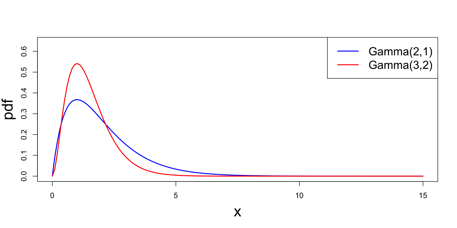
• In this case we write X \sim \Gamma(\alpha,\beta)

• \alpha is shape parameter

• \beta is rate parameter

Example - Gamma distribution

Plot

Plotting \Gamma(\alpha,\beta) for parameters (2,1) and (3,2)

Example - Gamma distribution

Expected value

Let X \sim \Gamma(\alpha,\beta). We have: \begin{align*} {\rm I\kern-.3em E}[X] & = \int_{-\infty}^\infty x f_X(x) \, dx \\ & = \int_0^\infty x \, \frac{x^{\alpha-1} e^{-\beta{x}} \beta^{\alpha}}{\Gamma(\alpha)} \, dx \\ & = \frac{ \beta^{\alpha} }{ \Gamma(\alpha) } \int_0^\infty x^{\alpha} e^{-\beta{x}} \, dx \end{align*}

Example - Gamma distribution

Expected value

Recall previous calculation: {\rm I\kern-.3em E}[X] = \frac{ \beta^{\alpha} }{ \Gamma(\alpha) } \int_0^\infty x^{\alpha} e^{-\beta{x}} \, dx Change variable y=\beta x and recall definition of \Gamma: \begin{align*} \int_0^\infty x^{\alpha} e^{-\beta{x}} \, dx & = \int_0^\infty \frac{1}{\beta^{\alpha}} (\beta x)^{\alpha} e^{-\beta{x}} \frac{1}{\beta} \, \beta \, dx \\ & = \frac{1}{\beta^{\alpha+1}} \int_0^\infty y^{\alpha} e^{-y} \, dy \\ & = \frac{1}{\beta^{\alpha+1}} \Gamma(\alpha+1) \end{align*}

Example - Gamma distribution

Expected value

Therefore \begin{align*} {\rm I\kern-.3em E}[X] & = \frac{ \beta^{\alpha} }{ \Gamma(\alpha) } \int_0^\infty x^{\alpha} e^{-\beta{x}} \, dx \\ & = \frac{ \beta^{\alpha} }{ \Gamma(\alpha) } \, \frac{1}{\beta^{\alpha+1}} \Gamma(\alpha+1) \\ & = \frac{\Gamma(\alpha+1)}{\beta \Gamma(\alpha)} \end{align*}

Recalling that \Gamma(\alpha+1)=\alpha \Gamma(\alpha): {\rm I\kern-.3em E}[X] = \frac{\Gamma(\alpha+1)}{\beta \Gamma(\alpha)} = \frac{\alpha}{\beta}

Example - Gamma distribution

Variance

We want to compute {\rm Var}[X] = {\rm I\kern-.3em E}[X^2] - {\rm I\kern-.3em E}[X]^2

• We already have {\rm I\kern-.3em E}[X]
• Need to compute {\rm I\kern-.3em E}[X^2]

Example - Gamma distribution

Variance

Proceeding similarly we have:

\begin{align*} {\rm I\kern-.3em E}[X^2] & = \int_{-\infty}^{\infty} x^2 f_X(x) \, dx \\ & = \int_{0}^{\infty} x^2 \, \frac{ x^{\alpha-1} \beta^{\alpha} e^{- \beta x} }{ \Gamma(\alpha) } \, dx \\ & = \frac{\beta^{\alpha}}{\Gamma(\alpha)} \int_{0}^{\infty} x^{\alpha+1} e^{- \beta x} \, dx \end{align*}

Example - Gamma distribution

Variance

Recall previous calculation: {\rm I\kern-.3em E}[X^2] = \frac{\beta^{\alpha}}{\Gamma(\alpha)} \int_{0}^{\infty} x^{\alpha+1} e^{- \beta x} \, dx Change variable y=\beta x and recall definition of \Gamma: \begin{align*} \int_0^\infty x^{\alpha+1} e^{-\beta{x}} \, dx & = \int_0^\infty \frac{1}{\beta^{\alpha+1}} (\beta x)^{\alpha + 1} e^{-\beta{x}} \frac{1}{\beta} \, \beta \, dx \\ & = \frac{1}{\beta^{\alpha+2}} \int_0^\infty y^{\alpha + 1 } e^{-y} \, dy \\ & = \frac{1}{\beta^{\alpha+2}} \Gamma(\alpha+2) \end{align*}

Example - Gamma distribution

Variance

Therefore {\rm I\kern-.3em E}[X^2] = \frac{ \beta^{\alpha} }{ \Gamma(\alpha) } \int_0^\infty x^{\alpha+1} e^{-\beta{x}} \, dx = \frac{ \beta^{\alpha} }{ \Gamma(\alpha) } \, \frac{1}{\beta^{\alpha+2}} \Gamma(\alpha+2) = \frac{\Gamma(\alpha+2)}{\beta^2 \Gamma(\alpha)} Now use following formula twice \Gamma(\alpha+1)=\alpha \Gamma(\alpha): \Gamma(\alpha+2)= (\alpha + 1) \Gamma(\alpha + 1) = (\alpha + 1) \alpha \Gamma(\alpha) Substituting we get {\rm I\kern-.3em E}[X^2] = \frac{\Gamma(\alpha+2)}{\beta^2 \Gamma(\alpha)} = \frac{(\alpha+1) \alpha}{\beta^2}

Example - Gamma distribution

Variance

Therefore {\rm I\kern-.3em E}[X] = \frac{\alpha}{\beta} \quad \qquad {\rm I\kern-.3em E}[X^2] = \frac{(\alpha+1) \alpha}{\beta^2} and the variance is \begin{align*} {\rm Var}[X] & = {\rm I\kern-.3em E}[X^2] - {\rm I\kern-.3em E}[X]^2 \\ & = \frac{(\alpha+1) \alpha}{\beta^2} - \frac{\alpha^2}{\beta^2} \\ & = \frac{\alpha}{\beta^2} \end{align*}

Moment generating function

• We abbreviate Moment generating function with MGF

• MGF is almost the Laplace transform of the probability density function

• MGF provides a short-cut to calculating mean and variance

• MGF gives a way of proving distributional results for sums of independent random variables

Moment generating function

Definition

The moment generating function or MGF of a rv X is M_X(t) := {\rm I\kern-.3em E}[e^{tX}] \,, \quad \forall \, t \in \mathbb{R}

In particular we have:

• X discrete: M_X(t) = \sum_{x \in \mathbb{R}} e^{tx} f_X(x)

• X continuous: M_X(t) = \int_{-\infty}^\infty e^{tx} f_X(x) \, dx

Moment generating function

Computing moments

Theorem

If X has MGF M_X then {\rm I\kern-.3em E}[X^n] = M_X^{(n)} (0) where we denote M_X^{(n)} (0) := \frac{d^n}{dt^n} M_X^{(n)}(t) \bigg|_{t=0}

The quantity {\rm I\kern-.3em E}[X^n] is called n-th moment of X

Moment generating function

Proof of Theorem

Suppose X continuous and that we can exchange derivative and integral: \begin{align*} \frac{d}{dt} M_X(t) & = \frac{d}{dt} \int_{-\infty}^\infty e^{tx} f_X(x) \, dx = \int_{-\infty}^\infty \left( \frac{d}{dt} e^{tx} \right) f_X(x) \, dx \\ & = \int_{-\infty}^\infty xe^{tx} f_X(x) \, dx = {\rm I\kern-.3em E}(Xe^{tX}) \end{align*} Evaluating at t = 0: \frac{d}{dt} M_X(t) \bigg|_{t = 0} = {\rm I\kern-.3em E}(Xe^{0}) = {\rm I\kern-.3em E}[X]

Moment generating function

Proof of Theorem

Proceeding by induction we obtain: \frac{d^n}{dt^n} M_X(t) = {\rm I\kern-.3em E}(X^n e^{tX}) Evaluating at t = 0 yields the thesis: \frac{d^n}{dt^n} M_X(t) \bigg|_{t = 0} = {\rm I\kern-.3em E}(X^n e^{0}) = {\rm I\kern-.3em E}[X^n]

Moment generating function

Notation

For the first 3 derivatives we use special notations:

M_X'(0) := M^{(1)}_X(0) = {\rm I\kern-.3em E}[X] M_X''(0) := M^{(2)}_X(0) = {\rm I\kern-.3em E}[X^2] M_X'''(0) := M^{(3)}_X(0) = {\rm I\kern-.3em E}[X^3]

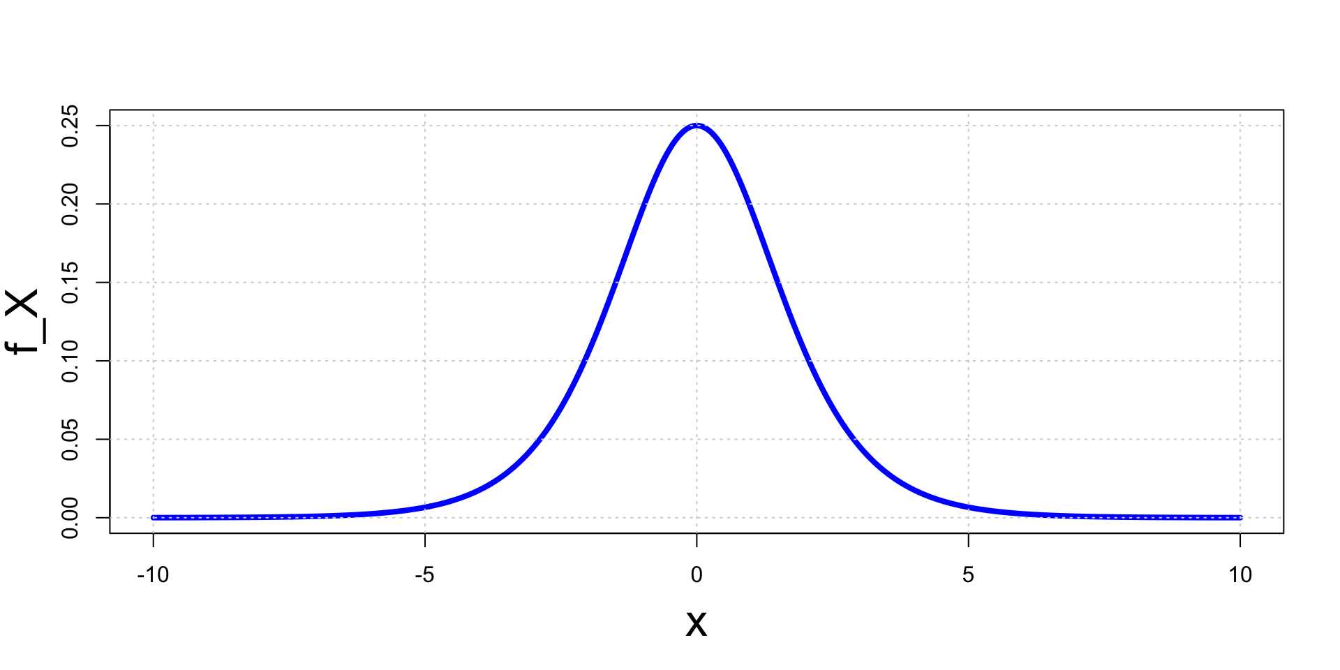
Example - Normal distribution

Definition

• The normal distribution with mean \mu and variance \sigma^2 is f(x) := \frac{1}{\sqrt{2\pi\sigma^2}} \, \exp\left( -\frac{(x-\mu)^2}{2\sigma^2}\right) \,, \quad x \in \mathbb{R}

• X has normal distribution with mean \mu and variance \sigma^2 if f_X = f

  • In this case we write X \sim N(\mu,\sigma^2)

• The standard normal distribution is denoted N(0,1)

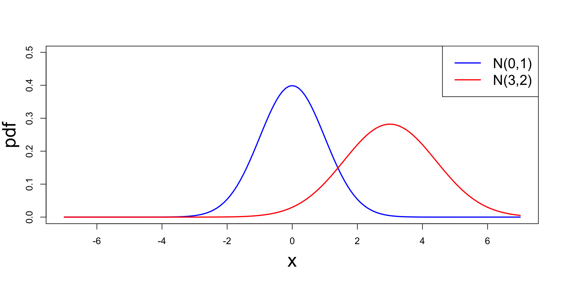
Example - Normal distribution

Plot

Plotting N(\mu,\sigma^2) for parameters (0,1) and (3,2)

Example - Normal distribution

Moment generating function

The equation for the normal pdf is f_X(x) = \frac{1}{\sqrt{2\pi\sigma^2}} \, \exp\left(-\frac{(x-\mu)^2}{2\sigma^2}\right) Being pdf, we must have \int f_X(x) \, dx = 1. This yields: \begin{equation} \tag{1} \int_{-\infty}^{\infty} \exp \left( -\frac{x^2}{2\sigma^2} + \frac{\mu{x}}{\sigma^2} \right) \, dx = \exp \left(\frac{\mu^2}{2\sigma^2} \right) \sqrt{2\pi} \sigma \end{equation}

Example - Normal distribution

Moment generating function

We have \begin{align*} M_X(t) & := {\rm I\kern-.3em E}(e^{tX}) = \int_{-\infty}^{\infty} e^{tx} f_X(x) \, dx \\ & = \int_{-\infty}^{\infty} e^{tx} \frac{1}{\sqrt{2\pi}\sigma} \exp \left( -\frac{(x-\mu)^2}{2\sigma^2} \right) \, dx \\ & = \frac{1}{\sqrt{2\pi}\sigma} \int_{-\infty}^{\infty} e^{tx} \exp \left( -\frac{x^2}{2\sigma^2} - \frac{\mu^2}{2\sigma^2} + \frac{x\mu}{\sigma^2} \right) \, dx \\ & = \exp\left(-\frac{\mu^2}{2\sigma^2} \right) \frac{1}{\sqrt{2\pi}\sigma} \int_{-\infty}^{\infty} \exp \left(- \frac{x^2}{2\sigma^2} + \frac{(t\sigma^2+\mu) x}{\sigma^2} \right) \, dx \end{align*}

Example - Normal distribution

Moment generating function

We have shown \begin{equation} \tag{2} M_X(t) = \exp\left(-\frac{\mu^2}{2\sigma^2} \right) \frac{1}{\sqrt{2\pi}\sigma} \int_{-\infty}^{\infty} \exp \left(- \frac{x^2}{2\sigma^2} + \frac{(t\sigma^2+\mu) x}{\sigma^2} \right) \, dx \end{equation} Replacing \mu by (t\sigma^2 + \mu) in (1) we obtain \begin{equation} \tag{3} \int_{-\infty}^{\infty} \exp \left(- \frac{x^2}{2\sigma^2} + \frac{(t\sigma^2+\mu) x}{\sigma^2} \right) \, dx = \exp \left( \frac{(t\sigma^2+\mu)^2}{2\sigma^2} \right) \, \frac{1}{\sqrt{2\pi}\sigma} \end{equation} Substituting (3) in (2) and simplifying we get M_X(t) = \exp \left( \mu t + \frac{t^2 \sigma^2}{2} \right)

Example - Normal distribution

Mean

Recall the mgf M_X(t) = \exp \left( \mu t + \frac{t^2 \sigma^2}{2} \right) The first derivative is M_X'(t) = (\mu + \sigma^2 t ) \exp \left( \mu t + \frac{t^2 \sigma^2}{2} \right) Therefore the mean: {\rm I\kern-.3em E}[X] = M_X'(0) = \mu

Example - Normal distribution

Variance

The first derivative of mgf is M_X'(t) = (\mu + \sigma^2 t ) \exp \left( \mu t + \frac{t^2 \sigma^2}{2} \right) The second derivative is then M_X''(t) = \sigma^2 \exp \left( \mu t + \frac{t^2 \sigma^2}{2} \right) + (\mu + \sigma^2 t )^2 \exp \left( \mu t + \frac{t^2 \sigma^2}{2} \right) Therefore the second moment is: {\rm I\kern-.3em E}[X^2] = M_X''(0) = \sigma^2 + \mu^2

Example - Normal distribution

Variance

We have seen that: {\rm I\kern-.3em E}[X] = \mu \quad \qquad {\rm I\kern-.3em E}[X^2] = \sigma^2 + \mu^2 Therefore the variance is: \begin{align*} {\rm Var}[X] & = {\rm I\kern-.3em E}[X^2] - {\rm I\kern-.3em E}[X]^2 \\ & = \sigma^2 + \mu^2 - \mu^2 \\ & = \sigma^2 \end{align*}

Example - Gamma distribution

Moment generating function

Suppose X \sim \Gamma(\alpha,\beta). This means f_X(x) = \begin{cases} \dfrac{x^{\alpha-1} e^{-\beta{x}} \beta^{\alpha}}{\Gamma(\alpha)} & \text{ if } x > 0 \\ 0 & \text{ if } x \leq 0 \end{cases}

• We have seen already that {\rm I\kern-.3em E}[X] = \frac{\alpha}{\beta} \quad \qquad {\rm Var}[X] = \frac{\alpha}{\beta^2}

• We want to compute mgf M_X to derive again {\rm I\kern-.3em E}[X] and {\rm Var}[X]

Example - Gamma distribution

Moment generating function

We compute \begin{align*} M_X(t) & = {\rm I\kern-.3em E}[e^{tX}] = \int_{-\infty}^\infty e^{tx} f_X(x) \, dx \\ & = \int_0^{\infty} e^{tx} \, \frac{x^{\alpha-1}e^{-\beta{x}} \beta^{\alpha}}{\Gamma(\alpha)} \, dx \\ & = \frac{\beta^{\alpha}}{\Gamma(\alpha)}\int_0^{\infty}x^{\alpha-1}e^{-(\beta-t)x} \, dx \end{align*}

Example - Gamma distribution

Moment generating function

From the previous slide we have M_X(t) = \frac{\beta^{\alpha}}{\Gamma(\alpha)}\int_0^{\infty}x^{\alpha-1}e^{-(\beta-t)x} \, dx Change variable y=(\beta-t)x and recall the definition of \Gamma: \begin{align*} \int_0^{\infty} x^{\alpha-1} e^{-(\beta-t)x} \, dx & = \int_0^{\infty} \frac{1}{(\beta-t)^{\alpha-1}} [(\beta-t)x]^{\alpha-1} e^{-(\beta-t)x} \frac{1}{(\beta-t)} (\beta - t) \, dx \\ & = \frac{1}{(\beta-t)^{\alpha}} \int_0^{\infty} y^{\alpha-1} e^{-y} \, dy \\ & = \frac{1}{(\beta-t)^{\alpha}} \Gamma(\alpha) \end{align*}

Example - Gamma distribution

Moment generating function

Therefore \begin{align*} M_X(t) & = \frac{\beta^{\alpha}}{\Gamma(\alpha)}\int_0^{\infty}x^{\alpha-1}e^{-(\beta-t)x} \, dx \\ & = \frac{\beta^{\alpha}}{\Gamma(\alpha)} \cdot \frac{1}{(\beta-t)^{\alpha}} \Gamma(\alpha) \\ & = \frac{\beta^{\alpha}}{(\beta-t)^{\alpha}} \end{align*}

Example - Gamma distribution

Expectation

From the mgf M_X(t) = \frac{\beta^{\alpha}}{(\beta-t)^{\alpha}} we compute the first derivative: \begin{align*} M_X'(t) & = \frac{d}{dt} [\beta^{\alpha}(\beta-t)^{-\alpha}] \\ & = \beta^{\alpha}(-\alpha)(\beta-t)^{-\alpha-1}(-1) \\ & = \alpha\beta^{\alpha}(\beta-t)^{-\alpha-1} \end{align*}

Example - Gamma distribution

Expectation

From the first derivative M_X'(t) = \alpha\beta^{\alpha}(\beta-t)^{-\alpha-1} we compute the expectation \begin{align*} {\rm I\kern-.3em E}[X] & = M_X'(0) \\ & = \alpha\beta^{\alpha}(\beta)^{-\alpha-1} \\ & =\frac{\alpha}{\beta} \end{align*}

Example - Gamma distribution

Variance

From the first derivative M_X'(t) = \alpha\beta^{\alpha}(\beta-t)^{-\alpha-1} we compute the second derivative \begin{align*} M_X''(t) & = \frac{d}{dt}[\alpha\beta^{\alpha}(\beta-t)^{-\alpha-1}] \\ & = \alpha\beta^{\alpha}(-\alpha-1)(\beta-t)^{-\alpha-2}(-1)\\ & = \alpha(\alpha+1)\beta^{\alpha}(\beta-t)^{-\alpha-2} \end{align*}

Example - Gamma distribution

Variance

From the second derivative M_X''(t) = \alpha(\alpha+1)\beta^{\alpha}(\beta-t)^{-\alpha-2} we compute the second moment: \begin{align*} {\rm I\kern-.3em E}[X^2] & = M_X''(0) \\ & = \alpha(\alpha+1)\beta^{\alpha}(\beta)^{-\alpha-2} \\ & = \frac{\alpha(\alpha + 1)}{\beta^2} \end{align*}

Example - Gamma distribution

Variance

From the first and second moments: {\rm I\kern-.3em E}[X] = \frac{\alpha}{\beta} \qquad \qquad {\rm I\kern-.3em E}[X^2] = \frac{\alpha(\alpha + 1)}{\beta^2} we can compute the variance \begin{align*} {\rm Var}[X] & = {\rm I\kern-.3em E}[X^2] - {\rm I\kern-.3em E}[X]^2 \\ & = \frac{\alpha(\alpha + 1)}{\beta^2} - \frac{\alpha^2}{\beta^2} \\ & = \frac{\alpha}{\beta^2} \end{align*}

Moment generating function

The mgf characterizes a distribution

Theorem

Let X and Y be random variables with mgfs M_X and M_Y respectively. Assume there exists \varepsilon>0 such that M_X(t) = M_Y(t) \,, \quad \forall \, t \in (-\varepsilon, \varepsilon) Then X and Y have the same cdf F_X(u) = F_Y(u) \,, \quad \forall \, x \in \mathbb{R}

In other words: \qquad same mgf \quad \implies \quad same distribution

Example

• Suppose X is a random variable such that M_X(t) = \exp \left( \mu t + \frac{t^2 \sigma^2}{2} \right) As the above is the mgf of a normal distribution, by the previous Theorem we infer X \sim N(\mu,\sigma^2)

• Suppose Y is a random variable such that M_Y(t) = \frac{\beta^{\alpha}}{(\beta-t)^{\alpha}} As the above is the mgf of a Gamma distribution, by the previous Theorem we infer Y \sim \Gamma(\alpha,\beta)

References

[1]

Bingham, Nicholas H., Fry, John M., Regression, linear models in statistics, Springer, 2010.

[2]

Fry, John M., Burke, Matt, Quantitative methods in finance using R, Open University Press, 2022.

[3]

Casella, George, Berger, Roger L., Statistical inference, second edition, Brooks/Cole, 2002.

[4]

DeGroot, Morris H., Schervish, Mark J., Probability and statistics, Fourth Edition, Addison-Wesley, 2012.

[5]

Dalgaard, Peter, Introductory statistics with R, Second Edition, Springer, 2008.

[6]

Davies, Tilman M., The book of R, No Starch Press, 2016.

[7]

Rosenthal, Jeffrey S., A first look at rigorous probability theory, Second Edition, World Scientific Publishing, 2006.